QuantRead
A structured reading path from crypto trader to quantitative systems builder.
This book is a curated collection of articles organized into a deliberate learning sequence. Each phase builds directly on the one before it — skipping ahead will leave gaps that compound into confusion later.
Who This Is For
Anyone who wants to:
- Trade crypto with a systematic, data-driven edge rather than gut feel
- Understand the mathematical foundations that institutional quants use
- Eventually build a personal quant system that generates trading signals automatically
The Five Phases
| Phase | Focus | Goal |
|---|---|---|
| 1 — Trading Foundations | Markets, price action, risk | Understand how markets work and how to survive in them |
| 2 — Trading Strategies | Momentum & mean-reversion | Execute real trades with clear edge and rules |
| 3 — Portfolio Construction | Diversification, Kelly, risk parity | Think in systems, not individual bets |
| 4 — Quant Foundations | Math, statistics, programming | Build the mathematical toolkit quant firms use |
| 5 — Quant Systems | Markov Chains, Neural Networks | Code systematic signal-generation models |
How to Use This Book
Read in order. Each article is a standalone piece but the sequence is intentional.
As you go through each phase, ask yourself: “Can I explain this concept to someone else without looking at notes?” If yes, move on. If not, re-read.
Phases 1–3 are about becoming a trader. Phases 4–5 are about becoming a quant.
The goal is to be both.
How to Start Learning to Trade
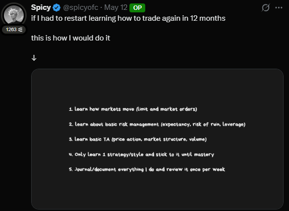
If I had to restart learning how to trade again in 12 months
- learn how markets move (limit and market orders)
- learn about basic risk management (expectancy, risk of ruin, leverage)
- learn basic TA (price action, market structure, volume)
- only learn 1 strategy/style and stick to it until mastery
- journal/document everything I do and review it once per week
1. Learn how markets move (limit and market orders)
Markets run on buyers and sellers placing orders. There are two basic order types:
- Market order — buy/sell immediately at the current price. Fast, but you have no control over your entry price.
- Limit order — place an order waiting at a specific price. More deliberate, lets you get a better price, but the order may never fill.
👉 Understanding these two order types = understanding how money flows in and out of the market.
2. Basic risk management (expectancy, risk of ruin, leverage)
- Expectancy — On average, does each trade make or lose money? A good strategy needs positive expectancy: profits outweigh losses over the long run.
- Risk of ruin — If you keep losing, how long before you run out of capital? Risk too much per trade → blow up fast, even with a good strategy.
- Leverage — Lets you trade with more than your actual capital. Bigger potential gains, but losses are multiplied equally. Misuse it and you self-destruct.
👉 Risk management matters more than strategy — lose less, stay in the game longer, and you give yourself a real chance to win.
3. Basic technical analysis (price action, market structure, volume)
- Price action — Read candlestick charts to understand market psychology: who is in control, buyers or sellers?
- Market structure — Is the market trending up, trending down, or ranging? Identify the bigger trend before entering a trade.
- Volume — Trading volume confirms the strength of a move. Price up + high volume = real move. Price up + low volume = be skeptical.
👉 These three elements help you read the market’s “language” instead of guessing.
4. Learn only one strategy/style and stick with it until mastery
Beginners often fall into “strategy hopping” — jumping to whatever looks good, never committing to anything long enough to get results.
Pick one approach (e.g. breakouts, support/resistance, trend following) → practice long enough → only then will you know if it actually works for you.
👉 Discipline matters more than finding the “perfect strategy.”
5. Document everything and review it once a week
A trading journal is the most powerful tool for improvement. Log: your reason for entering, your emotions at the time, the outcome, what went wrong. At the end of each week, sit down and review to find patterns in your own behavior.
👉 No journaling = no idea where you’re going wrong = repeating the same mistakes forever.
These five points are not about finding a “winning tip” — they are about building the foundation to survive and improve in trading over the long run.
Profitable Trading: Reverse Engineered
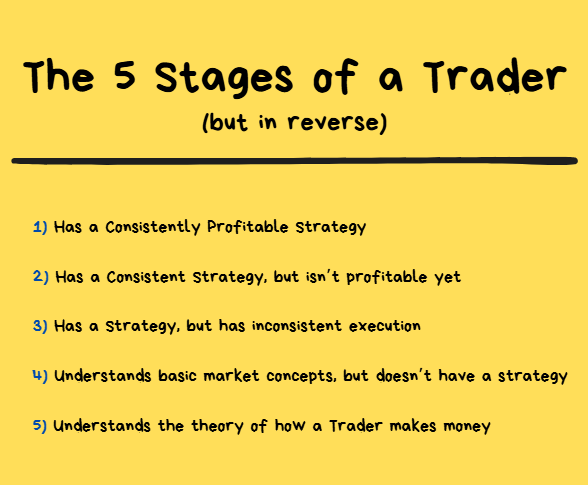
There are 5 Stages I went through from Unprofitable → Profitable.
I’m going to explain each of them below but in reverse.
I believe it will be easier to retain the information this way.
In this article I’m going to explain:
- Help you understand what a “constraint” is
- Explain each of the 5 stages starting from top to bottom.
- I will also explain what was the constraint that had to be solved in order to ascend to next stage
- Present my solution to each constraint at every single stage
I’m going to go pretty in-depth with everything here.
Let’s get started ↓
The 5 Stages and the Theory of Constraints
Remember we’re going to go in reverse with this article.
Defining “Constraint”:
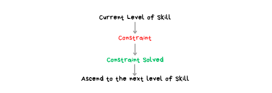
CONSTRAINT: The single biggest bottleneck holding a trader back from advancing to the next level of skill.
- It’s the one biggest problem that, if solved, makes everything else easier or unnecessary.
- An effective approach for improving at anything is identifying the biggest constraint and then pouring all focus, attention and resources into solving that specific constraint.
- This means tunnel vision focusing on solving 1 problem while ignoring all other problems.
In summary, at every stage a trader will need to identify their biggest constraint and continue to chip away at it until it is solved before they can ascend to the next stage.
Below I will get into each of the 5 Stages, their Constraints and how to Solve them. ↓
Stage 1 — Profitable Strategy

gentle reminder that we are reverse engineering this process and going backwards ;)
How to know you are at Stage 1:
• You have a strategy which can generate profits over a large # of trades.
• You have data to show that your strategy has a positive expectancy.
• You have some kind of process for improving your strategy and you have used this process many times already.
Stage 2 — Consistent but Not Yet Profitable
Let’s talk about the Stage that comes right before crossing over to becoming Profitable.

Every trade is being executed in the same way. The only issue is that the strategy isn’t actually making any money.
The point right before having a Consistently Profitable Strategy is having a Consistent Strategy but not necessarily Profitable.
How to know you are at Stage 2:
- You have a “consistent” trading strategy
- entry is the same on every trade
- exit is the same on every trade
- If you were to review 100~ trade screenshots they would all look pretty much the same.
This is the point where you have the skills to do market analysis + you have a strategy but money just isn’t coming in.
It can feel frustrating because it feels like “something is missing”.
That “something” is an “Improvement Process”
Explained below ↓
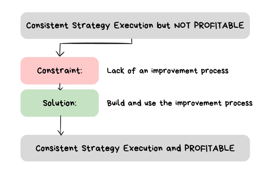
identifying the constraint and solution for Stage 2
QUESTION: What is the thing that MUST OCCUR in order to go from “a consistent strategy but it loses money” to “a consistent strategy but it makes money”?
ANSWER: An improvement process being used multiple times
Explanation
- Imagine a car is at Town A and needs to get to Town B which is 100km away.
- The car MUST BE MOVING in order to get to Town B. If it is standing still then it will not get to Town B.
- If the car is moving, regardless of how slow it is, it will eventually get to Town B.
The Point
- The ONE THING that matters the most at this stage is building an improvement process for your strategy and then using it as much as possible until eventually reaching profitability.
- It’s like having software which has 100 bugs in it. Build a process to identify each bug and fix each bug 1 at a time and eventually your software will work.
- This is a volume game. It’s unlikely that you are going to fix 1 issue with your strategy and magically become profitable.
- It’s more likely that you may need to fix 100+ things
The Solution: Building the Improvement Process
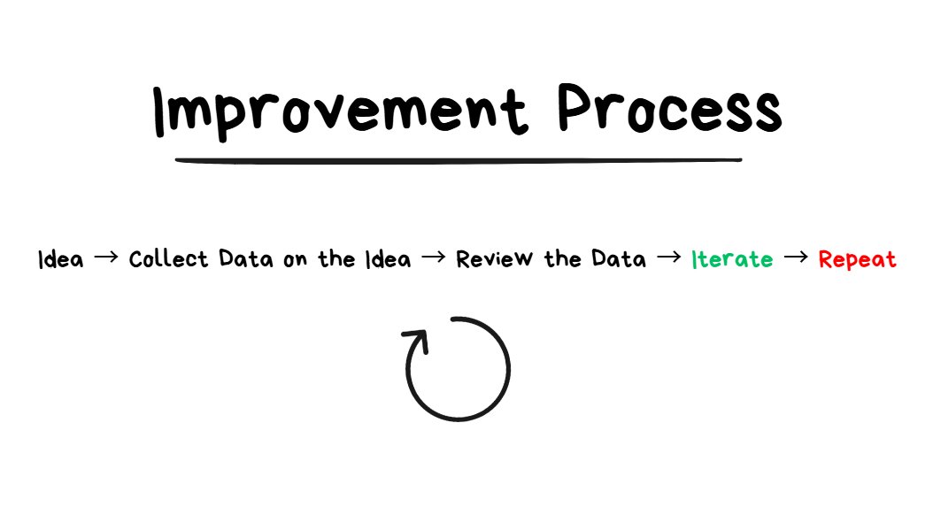
more repetitions with this loop = better ideas
better ideas = better iterations
There are 4 components to the improvement process:
- Idea (“I wonder if X will improve my winrate?”)
- Data Collection (see how many times X appeared in your trades)
- Review Data (see how much impact X had on the winrate)
- Iterate (based on the review, make a change to the trade execution next time X appears for a trade)
If you go through this feedback loop enough times then it is inevitable that you will perform better.
NON-TRADING EXAMPLE:
- Pretend I want to make a “cookie shop” which sells tasty cookies
- I bake 1 batch of cookies.
- I taste them, but feel like they’re not salty enough.
IDEA: I think they’re not salty enough. If I made them more salty then more people would like them.
DATA: I’m going to give my normal cookies and “slightly saltier” cookies to 100 different people and see which one they prefer.
REVIEW DATA: 73% of people prefer the salty cookies.
ITERATE: I will make a small adjustment to the recipe so that the cookies have a bit more salt in them based on the review of my data.
THE POINT: if I was to go through this same process and make 1,000,000 iterations I would have incredibly good tasting cookies by the end of it.
Important Reminder: Not All Reviews Will Find Alpha
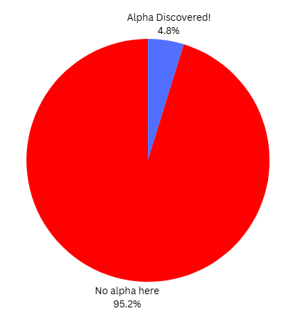
Only X% of your reviews will lead to finding “alpha” (a potential improvement in your strategy).
X is going to be a low number.
When you go through this “improvement process” multiple times you may find that a lot of the time you find yourself empty handed.
You had an idea, collected data on the idea, reviewed the data and it turns out there’s nothing special about the idea.
This doesn’t mean that “you suck” or that “your process is broken”.
This is just how things are. Edge is like a needle in a haystack. The sooner you accept this, the easier everything else will be.
When the above is understood, it then becomes clear that there are 4 things to be optimizing for:
- QUANTITY of data (how much data do you have)
- QUALITY of data (how statistically significant is the data)
- QUANTITY of reviews (how many reviews are you performing each month)
- QUALITY of reviews (increasing the likelihood of finding alpha within a review)
If you make ANY of these 4 go up, you will find MORE alpha.
This is a game of brute force.
Let’s use an extreme example:🤓
- You have 1,000,000,000 ideas about the market.
- You collect 1,000,000,000 data points on EACH idea.
- You review all 1,000,000,000 data sets
- 999,999,000 reviews end up going nowhere
- 1000 reviews end up finding real alpha
- If you have 1000 pieces of real alpha, you will become very profitable.
This should make it crystal clear that this is a game of brute force.
Get MORE ideas, TEST more ideas, REVIEW more ideas and you WILL FIND MORE ALPHA.
It sounds simple but it is hard and time consuming.
A Practical Improvement Process
So there’s really only 2 things that we can do to make more money:
- Option 1: Make MORE profitable decisions
- Option 2: Make LESS unprofitable decisions
The 2nd one is generally a lot easier to start with.
You can do literally EVERYTHING the same in your process but if you just make LESS MISTAKES then you will make MORE MONEY as a result of it.
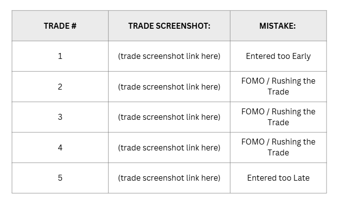
the easiest trade screenshot review you start with:
- finding trade execution mistakes
Before you start looking for super duper new Alpha, start with the raw basics.
- Identify every trade where you broke the rules of your trading strategy. Put all of those screenshots in a column of a spreadsheet. (it doesn’t even matter if the strategy is profitable or not. The point is you need to stick to the rules)
- Find the most common mistake
- Introduce an input which decreases the chance of the same mistake happening again.
Two Examples:
Entering too early? - use a checklist for all criteria that needs to be met
Entering too late? - use more alerts to give you more of a heads up that a potential trade is coming
Taking This Even Further
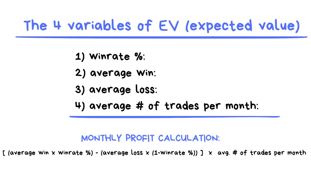
“the 4 variables of EV” and “the monthly profit equation”
After you have eliminated all mistakes from your execution the next step is to get creative.
You’re going to have to come up with ideas which impact any of these 4 variables in your strategy execution:
- Improve Winrate %:
This can be done by taking MORE GOOD TRADES or LESS BAD TRADES
2. Increase Average Win
This can be done by RISKING MORE ON GOOD TRADES or INCREASING THE WIDTH OF YOUR TARGETS
3. Decrease Average Loss
This can be done by CUTTING LOSERS EARLIER or REDUCING COSTS (fees/slippage)
4. Increase Trade Frequency
This can be done by INCREASING SCREENTIME , MORE/BETTER ALERTS and/or introducing MORE STRATEGIES into your toolbox.
From personal experience, this is the specific order I have found most effective to take for strategy improvement (based on amount of effort it takes to collect/review the data relative to the ROI of the insights gained from the dataset) :
- make fewer mistakes (increases winrate)
- take fewer low quality trades (increases winrate)
- cut losers faster on A+ setups (decreases avg. loss)
- risk more on A+ setups (increases avg. win)
- wider TP on A+ setups (increases avg. win)
- more/better alerts (increases frequency)
- introduce more strategies into toolbox (increases frequency)
If you use the Improvement Process Loop for 100 ideas on each of these 7 things it would be unreasonable to not find improvements within your execution.
Yes, this means coming up with 700 ideas, collecting 700 data sets, performing 700 reviews and iterating accordingly.
It’s simple but it takes effort and time.
Summary of Stage 2
If you have a strategy and you’re consistent with executing it but you’re NOT profitable yet, the thing that you’re missing is an improvement process. Use the “idea , collect data , review , iterate” loop to eliminate mistakes. Once all mistakes are eliminated, use the loop over and over again to make improvements to any of the big 4 variables in the EV equation which make up your monthly profit.
If you keep going through the loop you WILL find improvements and you WILL make more money.
Stage 3 — Inconsistent Strategy
Before having a consistent strategy, you must have an inconsistent strategy.

How to know you are at Stage 3:
You have a strategy but none of the trades look the same.
This is a problem because it makes Stage 2 harder to pass.
If every trade has different rules for entry, stoploss, target and management then it’s going to be really hard to find improvements.
Let’s use the Cookie Shop analogy again to explain how this is a problem:
- Imagine you bake 20 cookies.
- Each cookie has a different shape, size, color and flavor.
- If you try to put your cookies through the Improvement Process it will be too challenging to know what variable needs to be improved.
- 5 people might say too salty, 8 people might say too sweet, 3 people might say not sweet enough … the feedback from the data you collect will be all over the place and cannot be reliable because none of the cookies are the same.
- But if you bake the IDENTICAL cookie with ALL variables kept equal, you will be able to trust the data if 80% of people say “not salty enough”.
The Solution: Consistent Trade Execution
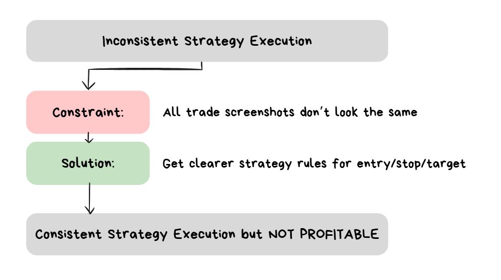
When all trade screenshots look pretty much the same, then the constraint has been solved.
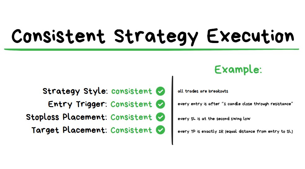
Consistency > Quality
FIRST make everything the same. You can optimize each of these LATER.
These problems I was facing while I was in this stage:
- I was trading BOTH breakouts and reversals, instead of just 1 style.
- I would be entering trades based on gut feel, instead of a clear entry trigger
- My stoploss would be placed at a place which “felt right” , instead of using a specific location every time.
- My target would also be based on gut feel, instead of using a specific target every time
The issue was that I was too short-sighted. I wanted to make money immediately and wanted to just skip over this step. If I thought it was good to trade reversals I would just trade reversals, if I thought it was good to trade breakouts I would trade breakouts… but from doing so many different things at the same time I was average at everything.
Mediocrity in Trading = NOT PROFITABLE.
🧠 SOLUTION = consistency. MAKE EVERYTHING THE SAME, DON’T WORRY ABOUT SHORT TERM RESULTS.
Eventually I realized that the only way that I could improve was to keep literally every single variable THE SAME and as SIMPLE AS POSSIBLE.
This means optimizing for CONSISTENCY rather than optimizing for RESULTS.
If execution IS NOT CONSISTENT but getting good results: then improving this strategy is going to be a really hard and slow process. I don’t want this. ❌
If execution IS CONSISTENT but not getting good results: then improving this strategy is going to be a fairly straightforward process. Even though short term results might suck, there’s a clear path forward for continuous iterations and fast learning/improvement. I want this. ✅
CONSISTENCY > SHORT TERM RESULTS
Summary of Stage 3
At this stage you have a strategy but the execution of the strategy is inconsistent and all over the place. In order to get over this stage you’re going to need consistent execution. This means same strategy style, same entries, same stoploss placement and same targets. If you want to get over this stage you’re going to have to let go of “perfection”. Accept that the short term results will suck, this is fine. The point is to make the strategy as EASY AS POSSIBLE to improve (by collecting lots of consistent data). The more identical your trade screenshots look, the easier the strategy will be to improve.
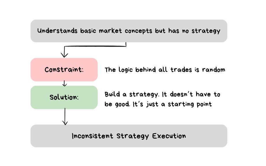
Stage 4 — No Strategy
Before having an inconsistent strategy, this is the stage of “having no strategy”.

at this stage understands basic technical analysis + risk management. The issue is just doesn’t know “what to actually do” in order to execute.
There are a lot of traders at this stage.
How to know you are at stage 4:
- You know some basic price action principles (e.g. bullish/bearish market structure)
- You know how to use an exchange and execute trades
- You know risk management basics
- But you DO NOT have any strategy with clearly defined rules for entry/stop/target/management.
The Solution: Having Some Strategy Rather Than None
something is better than nothing. This is not the time to worry about “quality” … (yet).
Without a strategy, throwing on longs/shorts blindly is really no different to going to a casino to gamble.
“Red or Black” v.s. “Up or Down” - same game, different name.
To overcome this stage a strategy needs to be built. Just SOMETHING. It doesn’t even have to be good. You can always “make it good” later.
Trying to immediately “make something good” with absolutely no reference points is foolish.
The Clay Pottery Class Analogy:
- A pottery teacher splits his class into 2 groups. Group A and Group B.
- Group A: their goal was to make the best looking clay pot in 30 days.
- Group B: their goal was to make as many clay pots as possible in 30 days.
- Result: Group B inevitably ended up making better looking clay pots (without even trying to) just because they had more repetitions and iterations.
- The point: get a high volume of reps FIRST. Do optimization SECOND.
The Four Components of a Trading Strategy
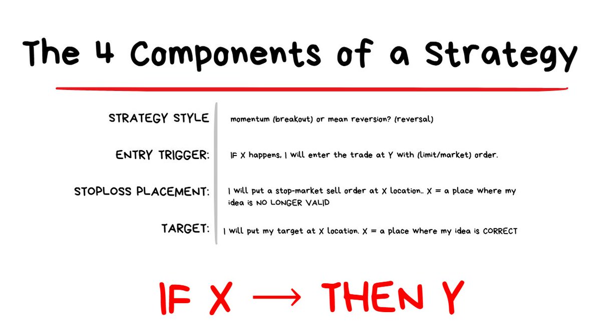
each component of a strategy follows a “IF X –> THEN Y” framework.
If X happens –> then I will do Y action.
If X does not happen –> then I will not do Y action.
STRATEGY STYLE: Momentum or Mean Reversion
- Momentum = betting that price will “break” a level
- Mean Reversion = betting that price will “reverse” from a level
- You’re going to have to pick if you want to trade Momentum or Mean Reversion to start off with.
- It doesn’t matter which one you pick because in the long term you will inevitably learn how to trade both.
- I recommend starting with Momentum because it’s easier and there are less variables you have to consider.
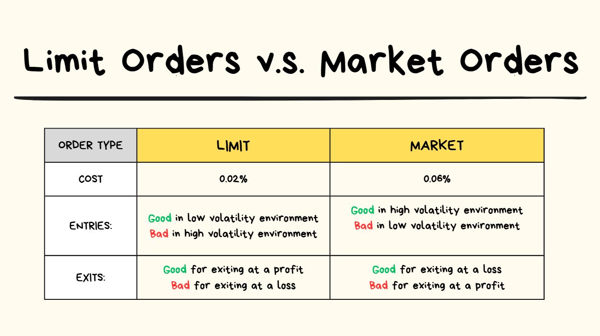
ENTRY TRIGGER: if X happens, I will place my entry at Y using (limit/market) order.
- The more simplistic the approach you have for defining X and Y, the easier everything else will be.
- Remember, simple is best at this stage. It’s not about finding the winning combination yet. It’s about having something that will be EASY to collect data on and EASY to iterate/improve.
- I suggest starting with limit order entries.
- Accept that you will miss some winning trades when using limit orders for entry. This is a feature, not a bug.
- As long as missed trades are journaled it will be easy to review them and easy to introduce market orders to start catching some of those missed trades.
STOPLOSS PLACEMENT: If X happens, I will put my stop-market sell order at Y location.
If going LONG = place stoploss at a swing low.
If going SHORT = place stoploss at a swing high.
❗️NOTE TO READER: will discuss market structure + price action concepts a bit further down below.
TARGET PLACEMENT: If price reaches X = my idea is correct.
- Assume that the first attempt of creating this rule for your target placement is NOT GOING TO BE OPTIMAL.
- It’s either going to be TOO WIDE or TOO TIGHT.
- Question: If I had to pick, would I rather have a TP that is too wide or too tight?
- Answer: Too tight.
- Reasoning: to improve a tp that is too tight you just have to look at winning trade screenshots where price extended beyond the TP by “N units of R” and then optimise from there. It’s straightforward. However to improve a tp that is too wide you have to look at losing trade screenshots where price went N units of R onside and then turned around and turned into a losing trade. It’s a tougher process.
Further Reading: Momentum Trading Strategy
Jul 31, 2025
Summary of Stage 4
If you have no strategy, the only way to move forward is to build a strategy. Something is better than nothing. Get some rules in place for the Strategy Style, Entry Trigger, Stoploss Placement and Target Placement. Don’t waste time trying to optimize it or make it perfect. Just build SOMETHING. After you have SOMETHING, you can go and optimize it AFTER you collect some data with using it.
The constraint is solved as soon as you can clearly state the rules of your strategy.
Stage 5 — Learning the Basics
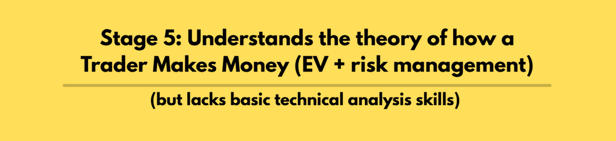
The trader knows what “expected value” is and understands that the goal of a trader is to capture as much of it as possible.
The trader just has no idea where to start with the basics of the technicals.
It’s not about winning the next trade. It’s about having a profit over the next N number of trades, where N is a large value.
How to know you are at Stage 5:
- You understand the importance of having an Edge
- You understand what Expected Value (EV) is
- You know basic Risk Management concepts
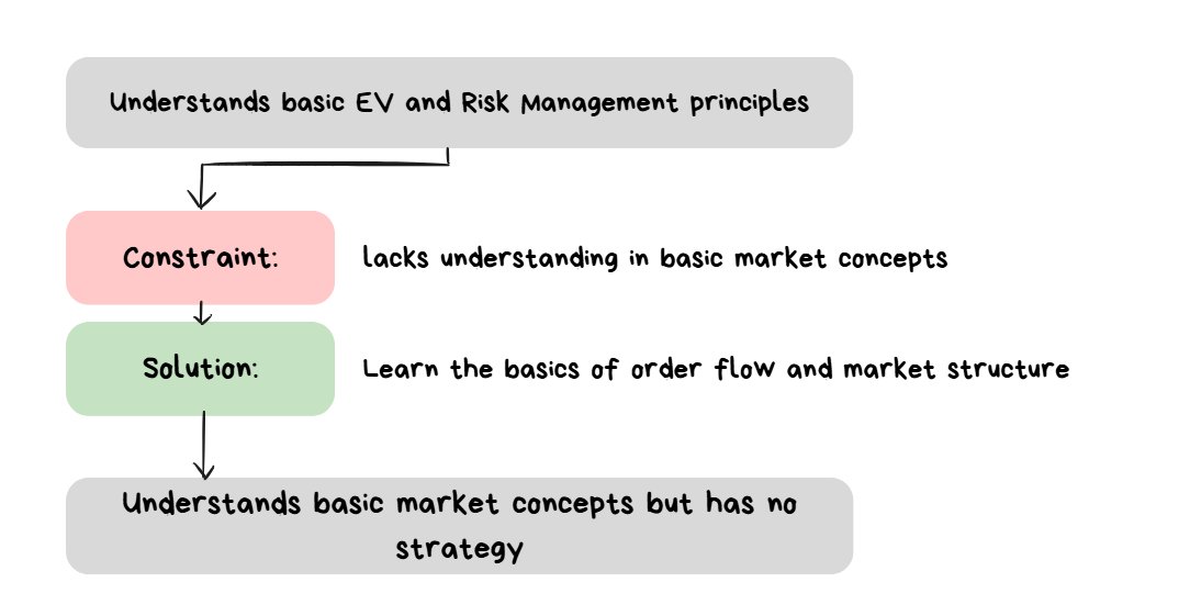
Before building a strategy, a Trader has to at least understand the basics of how markets move and some basic price action concepts.
The Solution: Learning Market Structure + Price Action Basics
Before getting into the practical (actually doing stuff), one has to learn at least some basic theory (how stuff works).
These are the 2 Topics I will cover below:
-
- How do markets move (market/limit orders basics)
-
- market structure + regimes basics
You don’t have to remember each and every single detail. It is more important to just understand the basic concepts.
After a basic understanding of the concepts is achieved does it make sense to start looking into building a strategy.
1) How Do Markets Move?
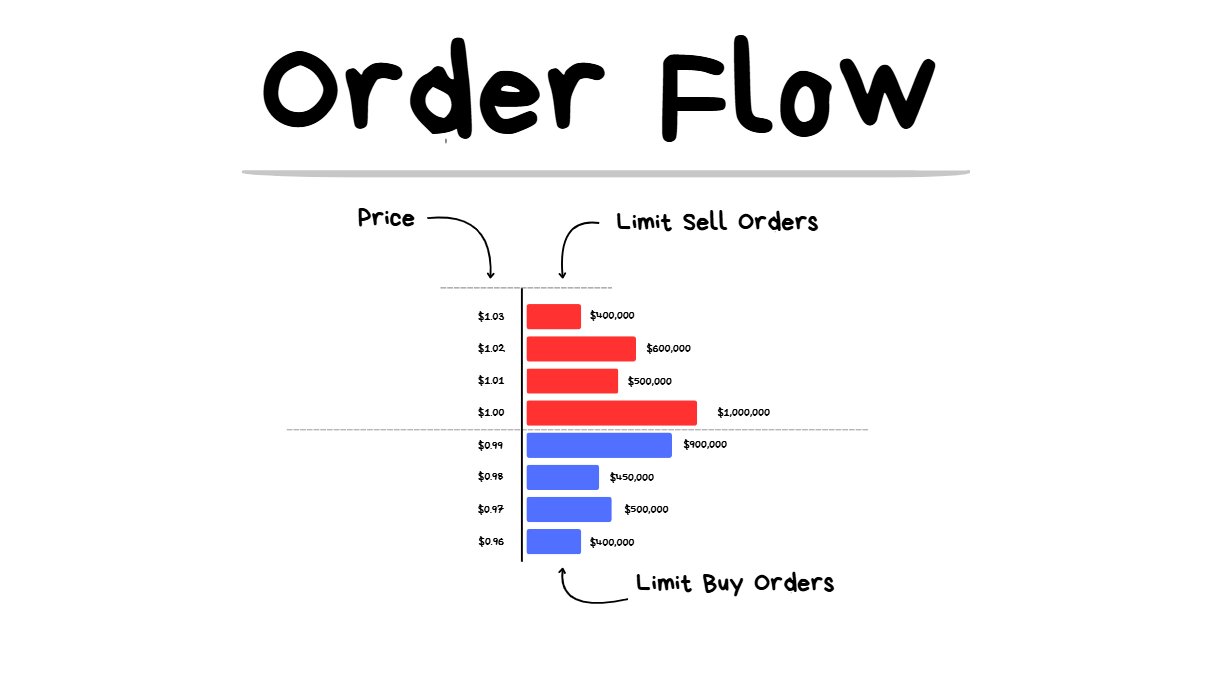
order book
The two order types:
- Limit Orders (I am advertising to execute a trade at X price. My trade will only execute if another participant wants to execute at my price.)
- Market Orders (I want to execute a trade NOW. I will pay an extra fee to get my trade executed immediately at whatever the best available current price is.)
Example using Apples: 🍎🍎🍎🍎🍎
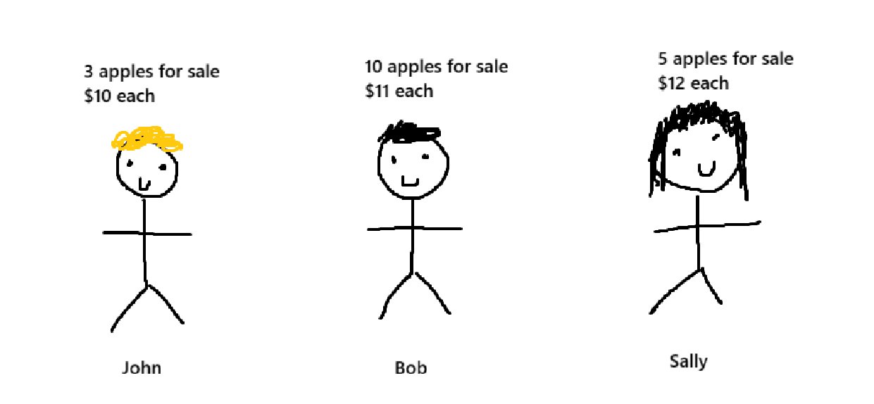
admire my beautiful creation on MS paint while you learning about order flow basics
If you want to buy 1 apple NOW (market buy) , you will buy 1 apple from John at $10 since $10 is the cheapest “limit sell order) available at the moment.
The last traded price of “apples” will be $10.
Then you realize you actually needed 4 more apples to bake your apple pie, so you go out and “market buy” 4 apples.
You instantly buy the 2 remaining apples from John at $10 each. John has now sold out of apples.
The next best available price for apples is $11 and Bob has 10 apples for sale. So you buy 2 apples from Bob at $11 each. Bob now has 8 apples remaining at $11 each.
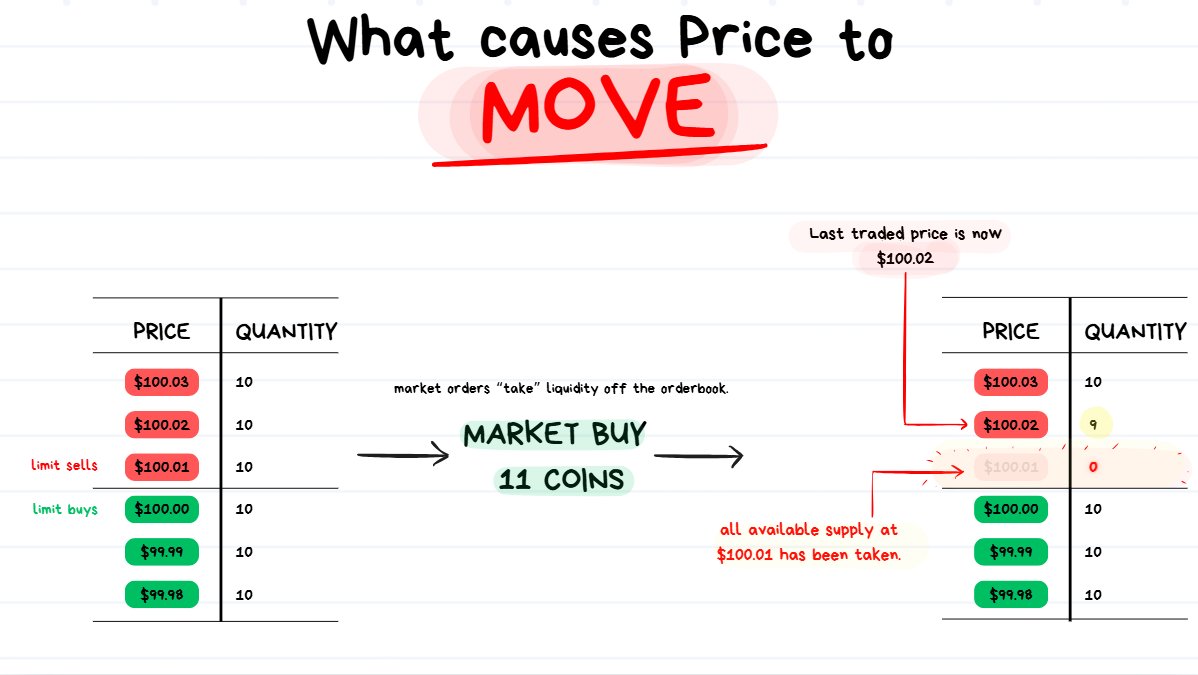
So what happened:
- you “market buy” 1 apple, price = $10
- you “market buy” 2 apples, price = $10 (all available supply is gone now)
- you “market buy” 2 apples, price = $11 (you pushed the price up)
A common Question that is often asked by traders is “Why did the Price go from A to B?”
- The only correct fundamental answer to this question is “because a bunch of market orders came through”
- There are an infinite # of possible reasons as to WHY traders were buying/selling. Some Examples: reacting to news, hedging a position, speculating on price action, arbitraging, blatant gambling etc.
- But we can never truly know the “why” because there will always be X% of information that is unaccountable for and impossible to collect/track/review.
- The only thing that we really know is that “market orders executed against resting limit orders, pushing the price from A to B”
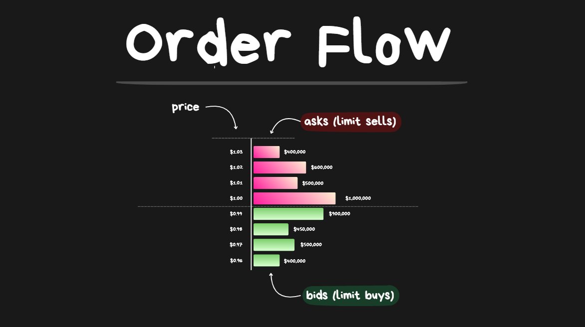
Behind all the fancy indicators and lines on a chart is just an order book filled with makers (people who are advertising to buy/sell with limit orders) and takers (people who bite on the advertisement and execute a market order).
Ultimately, everything comes down to these 2 things:
- How much $ is there in limit orders? (supply)
- How much $ is coming through in market orders? (demand)
2) Market Structure + Regime Basics
Below I’m going to cover the following:
- Swing Highs and Swing Lows
- Bullish/Bearish Market Structure
- Breaks of Market Structure
- What is a Regime (market environment)
- Regimes on a “continuum”
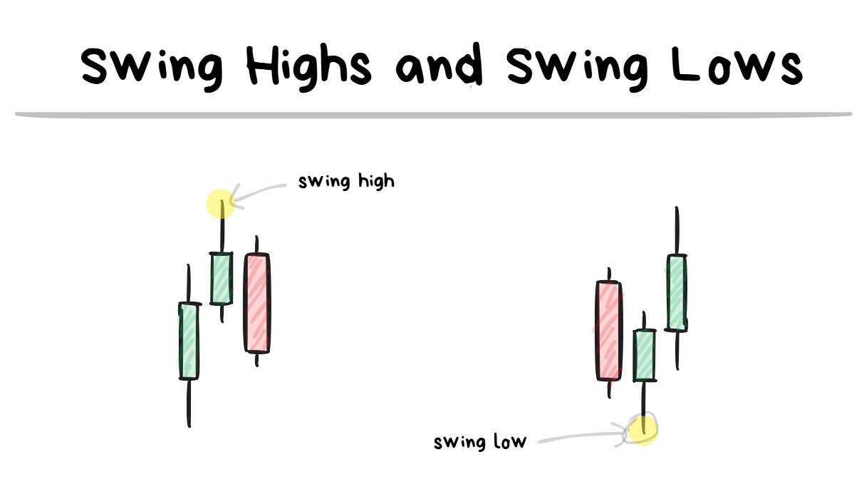
swing high/lows are turning points on the chart.
a low will look like a “V” and a high will look like an “upside-down V”
I believe the swing highs/lows are pretty self explanatory.
They are just previous turning points on the chart.
It requires at least 3 candles to form a swing level with the “extreme” being the level I look at.
the highs/lows in the diagram above are referring to “swing highs” and “swing lows”.
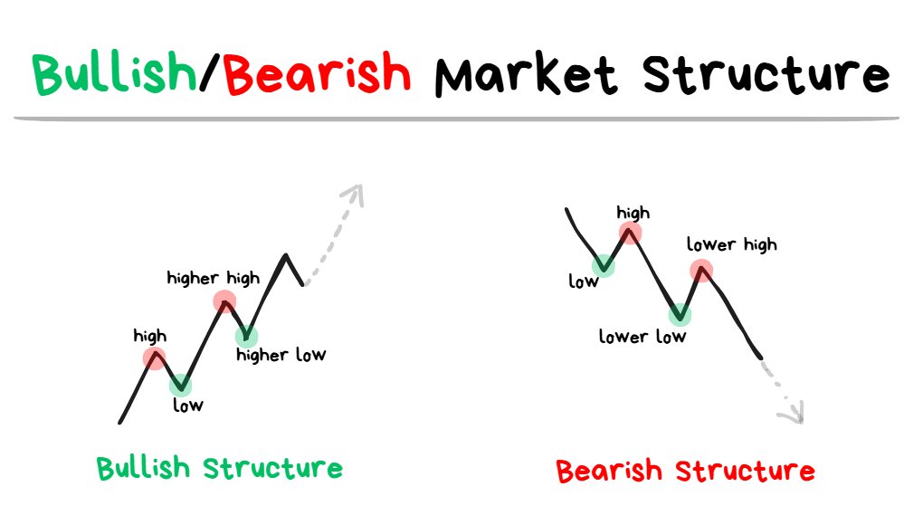
🐂Bullish Market Structure:
- Has higher highs and higher lows
- Expecting higher prices as long as structure remains in tact.
🐻Bearish Market Structure:
- Has lower highs and lower lows
- Expecting lower prices as long as structure remains in tact.
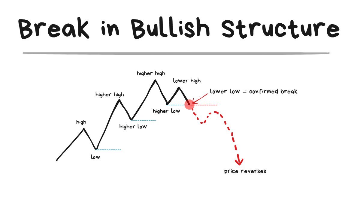
Break of Bullish Structure:
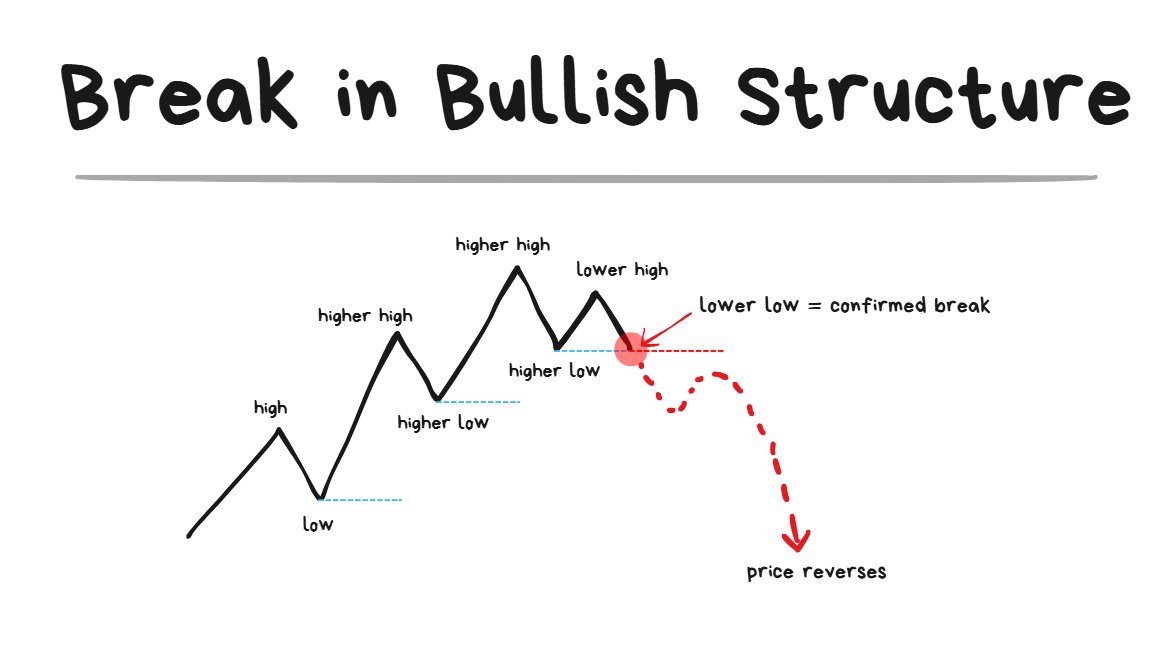
once the Lower Low comes in = the structure has broken.
- Just because a Lower High comes in does NOT mean the structure has broken yet
- The structure is only broken when the Lower Low comes in.
- A Lower Low = the breach of the most recent swing low that was formed.
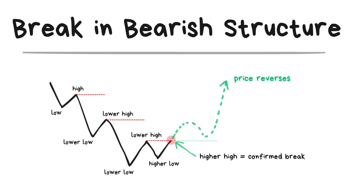
Break of Bearish Structure:

Once the Higher High comes in = the structure has broken
- Just because a Higher Low comes in does NOT mean the structure has broken yet.
- The structure is only broken when the Higher High comes in.
- A Higher High = the breach of the most recent swing high that was formed.
What Is a Regime?
A “Regime” is just a way to define a specific type of market environment.
Some regimes are more suitable for one style of strategies and other regimes are more favorable for other types of strategies.
Since market conditions change all the time, a big part of being a trader is being able to recognize the changes in regimes and adapt accordingly.
Jul 21, 2025
Creating a Market Bias If in sync: • risk more + trade more If out of sync: • risk less + trade less ↓
I like to have 2 types of biases I like to use:
- Directional (favored for longs or shorts?)
- Structural (favored for breakouts or reversals?)
If you were to look at any price action chart you may notice that a Break of Structure isn’t 100% guaranteed to result in a reversal.
Sep 10, 2025
My 2 favorite Trading setups ↓
In a Strong Bullish Trend: ❌
- as soon as price comes into the swing low, traders will quickly jump in to buy the discounted coin and price will accelerate higher.
- Betting on a reversal on a break of structure will NOT be ideal.
- Same logic applies to strong bearish trends too.
In a Weak, Sideways Choppy Range: ✅
- Price will continuously fail to break out of the major key levels
- As soon as the break of structure comes after the failure, the reversal is a lot more reliable.
The point: don’t obsess and try trade every single structural break. You’ll get burnt doing this in the wrong market environment. These work best in sideways environments.
Regimes on a Continuum
Sep 2, 2025
The 2 main Trading Styles I rely on explained↓
It’s not as simple as labelling a regime in a binary way. I’ve found it more helpful to think in terms of a continuum.
Examples:
- Sure a regime can be good for longs, but HOW GOOD is it?
- Sure a regime can be favorable for momentum trades, but HOW FAVORABLE is it?
- Sure price action can look choppy, but HOW CHOPPY is it?
The more clearly you can define the start/end points of a regime and also the changes in regimes = the easier trading will be.
Most traders obsess about optimizing their trading strategy but optimizing how you read the current market conditions (regime) is going to take you much further.
Summary of Stage 5
Once you understand the basics of Expectancy and Risk Management the next step is to learn the basics of price action.
Understanding how markets move with limit/market orders + market structure + regimes is a solid foundation to have.
Just remember:
- Directional Bias: up/down
- Structural Bias: trendy/choppy
If you can get a basic read on both then you can start developing a trading strategy to specifically take trades in 1 of those regimes.
Conclusion
Before you can have a profitable trading strategy, you will need a consistent trading strategy (which doesn’t need to be profitable yet).
In order to get from consistent strategy (unprofitable) to consistent strategy (profitable) you will need an “improvement process” where you come up with ideas, collect data on those ideas, review the data and make iterations accordingly.
Before you can have a consistent strategy (unprofitable) you will need to have some kind of strategy (but it doesn’t have to be consistent). The way to go from inconsistent to consistent is to get clearer definitions on your entry/exit rules + get a bit more systematic with the trade execution.
Before building a strategy you’re going to need to learn the absolute basics of how markets move (limit/market orders) and some price action basics. Your strategy should be built around performing well in ONE specific regime.
Final Words
Well done for pushing through this article. This was a pretty lengthy one.
Now you should have a bit more clarity on how my own trading journey looked like and maybe you can use parts of it as inspiration to replicate in your own.
If you really did take the time to read through this, then don’t hesitate to comment any questions.
I will take my time to go through ALL questions you guys put into the comments. Don’t be shy.
Good luck trading~ 🤝
Source
Written by @spicyofc · View original post · Published: 2025-07-31 �������������������������������������������������������������������������������������������
Price Action + Market Structure Masterclass

I’m a former Prop Trader and I’ve been trading Crypto for 8 years.
Basic understanding of price action concepts is something that every good trader that I’ve spoken to has in common.
So the goal of this article is to try simplify the basics and pass it over to you. 🤝
Here is everything that you’re going to get in this Article ↓
- Lesson 1: How does Price actually move?
- Lesson 2: Support and Resistance
- Lesson 3: Ranging Structure and Trending Structure
- Lesson 4: Live Trade Examples + 5 Bonus Resources
**🤓**NOTE TO READER: I have done my best to simplify all of these concepts as much as possible. Enjoy~
Lesson 1: How Does Price Actually Move?
orderbook
🤓NOTE TO READER: There is a reason why I want to cover this lesson first.
Unfortunately the majority of Traders don’t actually understand the causes for price moving up/down.
There are even some Traders out there who believe that the elites of society created a dark secret predatory algorithm which controls all the price movements in the market and it is designed to hunt stoplosses at certain times of the day….(yes seriously… there are surprisingly a large number of people out there who actually believe this.)
I can assure you, the market is not a “super coded algorithm by the elites”… it is a lot more like an auction at eBay.
If the most basic understanding of markets is incorrect or misguided, then all other ideas that the trader is going to come up with are going to be sitting on a very unstable foundation.
The goal of this lesson is to at least get the basics right. That’s it.
Okay let’s jump into the lesson ↓
This lesson will cover:
- What even is a “Market”
- Makers and Takers (limit orders/market orders)
- What causes the price to move and how does it happen
What Even Is a “Market”?
As soon as someone is willing to buy something, a market now exists for that something.
- If someone wants to buy a specific Pokemon card, then there is a “market” for that specific Pokemon card.
- If someone wants to buy an apple, then there is a “market” for apples.
- If someone wants to buy a burger, then there is a “market” for burgers.
- If someone wants to buy crypto shitcoins, then there is a “market” for crypto shitcoins.
A thing doesn’t need to be listed on an exchange with fancy candlestick charts and liquidity providers for it to have a market.
As long as someone wants to buy something then a market technically exists for it.
Makers and Takers (Limit Orders / Market Orders)
order types cheat sheet
In ALL markets there are Makers and Takers.
Maker:
- someone who is advertising to buy or sell “something” at a specific price.
- Example: “Bob is willing to sell 2 apples for $1 each.”
- The Maker may need to patiently wait for another market participant to see their advertisement and make a transaction with them.
Taker:
- The Taker is someone sees the advertisement of the Maker and agrees to the price.
- They will make the transaction with the Maker at whatever price the Maker wanted.
- But the Taker gets to decide on the quantity of how much of the thing they wanted to transact.
- Example: “Timmy agrees to Bob’s price of apples at $1 each, but Timmy only purchases 1 apple. Timmy gives Bob $1 and immediately receives 1 apple in exchange.”
In the Crypto Markets, “Makers” are those who are putting limit orders onto an orderbook. If you were to put in a “limit buy order for 1 BTC at $90,000” then you order will be sitting on the orderbook until price drops down to it.
❗️TIP: “Liquidity” is just a fancy way of saying “how much money is there sitting in limit orders.”
“Takers” are the ones who will be using market orders to execute against the resting limit orders. When you execute a Market Order, you don’t get to choose the price that you get. If you want to “market sell 1 BTC”, your order for 1 BTC will execute at whatever the best limit buy orders are available at the time.
What Causes Price to Move?
Market moves based on Supply and Demand at certain price points.
- Supply = Limit Orders (from makers)
- Demand = Market Orders (from takers)
Below I’m going to explain Supply/Demand using an analogy with Apples 🍎↓
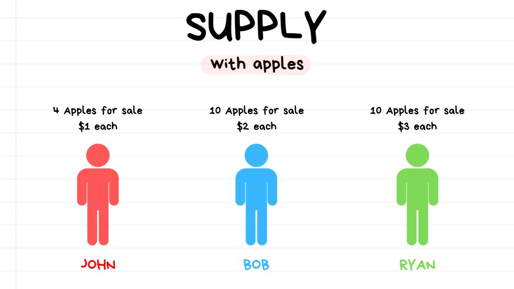
3 traders providing liquidity to apples. (supply)
There are 3 Makers (advertising to sell a specific price/quantity) for Apples:
- John has 4 apples for sale at $1 each.
- Bob has 10 apples for sale at $2 each.
- Ryan has 10 apples for sale at $3 each.
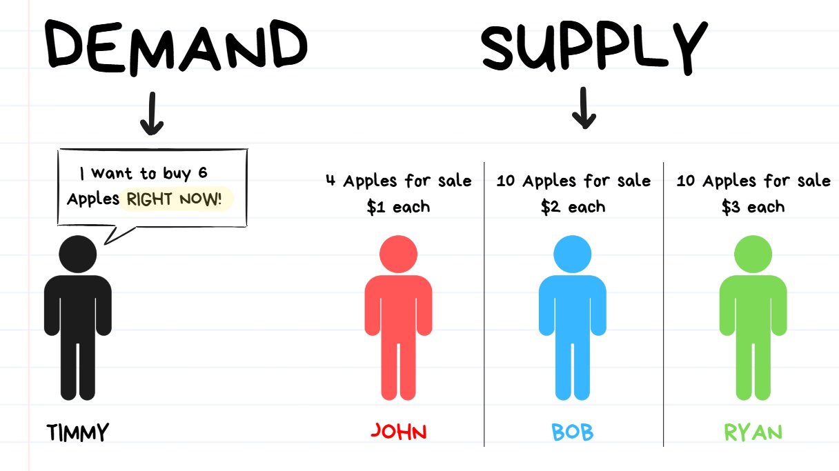
a taker (demand, in the form of market orders) has appeared.
↑ Timmy the Taker has appeared!
Timmy wishes to buy 6 apples immediately. He doesn’t care what price he gets, he just needs 6 apples to cook the best apple pie.
In order for Timmy to act on his intent, he will need to execute a Market Buy for a quantity of 6 apples.
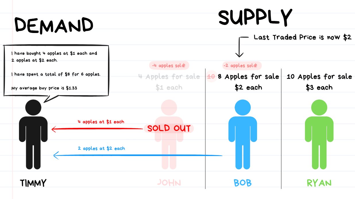
market order for 6 apples has been executed. price moves from $1 up to $2.
Once Timmy executes a Market Order for a quantity of 6 apples, this is what will happen:
- First Timmy’s order will take from the best available limit sell order. This will be the 4 apples from John at $1 each.
- However since John only has 4 apples for sale and Bob wants 6, Bob will eat through ALL of Bob’s supply. Timmy still has 2 apples left to buy.
- The next best available price will be $2 each from Bob. So Timmy will purchase the last 2 apples from Bob.
So Timmy bought 4 apples at $1 each ($4 of liquidity taken) and took all the available supply.
Then Timmy bought another 2 apples at $2 each from Bob ($4 of liquidity taken).
So BEFORE Timmy placed the order, the price of apples was $1.
AFTER Timmy’s Market order finished executing, his order resulted in pushing the price from $1 up to $2 because he ate through all the supply.
❗️TIP: So basically whenever demand exceeds supply at a certain price point, the price will move.
Summary: Lesson 1
Price doesn’t move because of secret algorithms. It moves because of supply and demand between buyers and sellers.
- Markets: A market exists anytime someone wants to buy or sell something. It can be apples, Pokémon cards, or Crypto.
- Makers (limit orders): Provide liquidity by advertising prices they’re willing to buy/sell at.
- Takers (market orders): Remove liquidity by accepting those prices immediately.
Price moves when market orders (demand) consume the available limit orders (supply) at a given price. If a large market buy eats through all sell orders at $1 and starts filling $2 orders, the price rises to $2.
👉 In short: Price = the result of market orders hitting the orderbook.
Lesson 2: Support and Resistance
The topic of support/resistance is a rather simple topic.
Unfortunately, Traders have a unique talent for finding ways to overcomplicate basic concepts and confuse themselves in the mess that they have created.
The goal of this lesson is get crystal clear clarity on Support/Resistance and remove any potential confusions.
This lesson will cover:
- Stop thinking about Magical Lines, start thinking about Limit Orders
- Order Size relative to Volatility
- Swing Highs and Swing Lows
Stop Thinking About Magical Lines, Start Thinking About Limit Orders

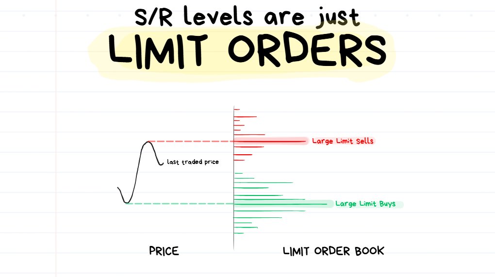
price isn’t bouncing from the lines you draw. It’s bouncing from limit orders in the orderbook.
Out in the vast space of social media are a whole bunch of influencers who try to create fancy-sounding ways of drawing different types of support/resistance levels.
Behind all the fancy “order blocks” and “price delivery zones” (or whatever other terms are used) is literally just a bunch of limit orders.
Ultimately, as discussed in the previous lesson, price moves purely based on Limit Orders and Market Orders.
So price is never bouncing off the “magical lines” (or boxes) that you draw on your chart. It is bouncing off the limit orders on the orderbook.
❗️****TIP: The lines that we draw on the chart are just to help us visualize where large clusters of limit orders are sitting.
You will often find big clusters of Limit Orders near previous big turning points in the price action.
The thing is I could draw a random line anywhere on the chart and behind it are probably going to be some limit orders.
This means you can draw literally any line on your chart and you could technically call it a valid support or resistance level.
Order Size Relative to Volatility
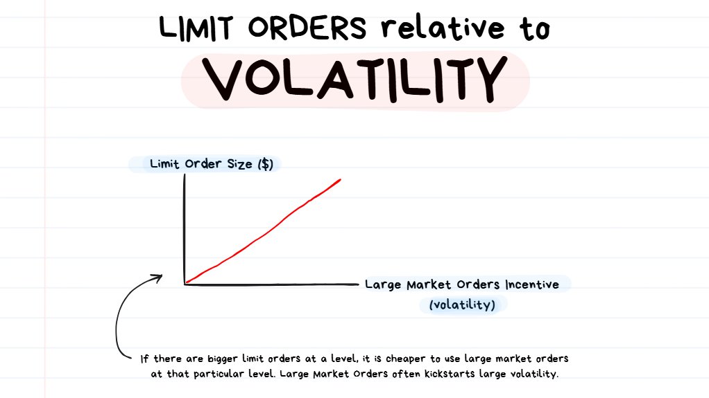
The bigger the advertisement, the louder the market gets after a sale occurs.
If there’s a lot of money in limit orders at 1 price, there’s more incentive to use market orders at that point since the slippage for large orders is at its lowest.
Since market orders are responsible for moving price up/down, we can expect to see a lot of movement once price hits a large limit order and starts moving away from it.
- This means that sometimes price can come into an “interesting looking” level but it just has very few limit orders there… meaning it’s not likely to have a violent reaction to the level.
- This also means that a big limit order can be placed at a very strange and unexpected place in the chart and have a big impact on price action once the price reaches that point.
Quick Summary (with a Hot Take🔥)
So basically there’s no such thing as “strong levels” or “weak levels”… yep I’ve said it. 🤷♂️
It’s not about “weak” or “strong”, it’s just about how much $$ in limit orders is sitting at a level relative to the other nearby limit orders.
More money sitting at a level in limit orders does not necessarily mean a higher likelihood of a “bounce” from the level (which is most commonly assumed).
It just means that we can expect to see a more volatile reaction once price gets closer to the level since big limit orders often incentivize big market orders to come through, which then cause big price movements.
- This means if a reversal happens from a level with huge orders, it’s likely to be a very violent reversal.
- If a breakout happens at the level with huge orders, it’s likely to be a very violent breakout.
If there’s very small limit orders at a level, then regardless if the price reverses or does a breakout it’s unlikely to be a wild move because there just isn’t “that much fuel for the fire to use.”
🧠3 BONUS TIPS ↓
❗️TIP #1: Big/Round Numbers which are in multiples of 10 (e.g. $1, 10, $10, $50… etc.) often have large limit orders stacked on them. This is why we see frequent violent reactions from these levels.
❗️TIP #2: For more advanced (or curious) Traders, you can use the platform @tapesurfapp to see where the limit orders are. I’m not affiliated with them in any way, I just think their platform is super cool.
❗️TIP #3: The more time that price has spent away from a level = the more time the market as a whole has to place limit orders at that level = the bigger the reaction can be expected once price returns to that level again.
Swing Highs and Swing Lows
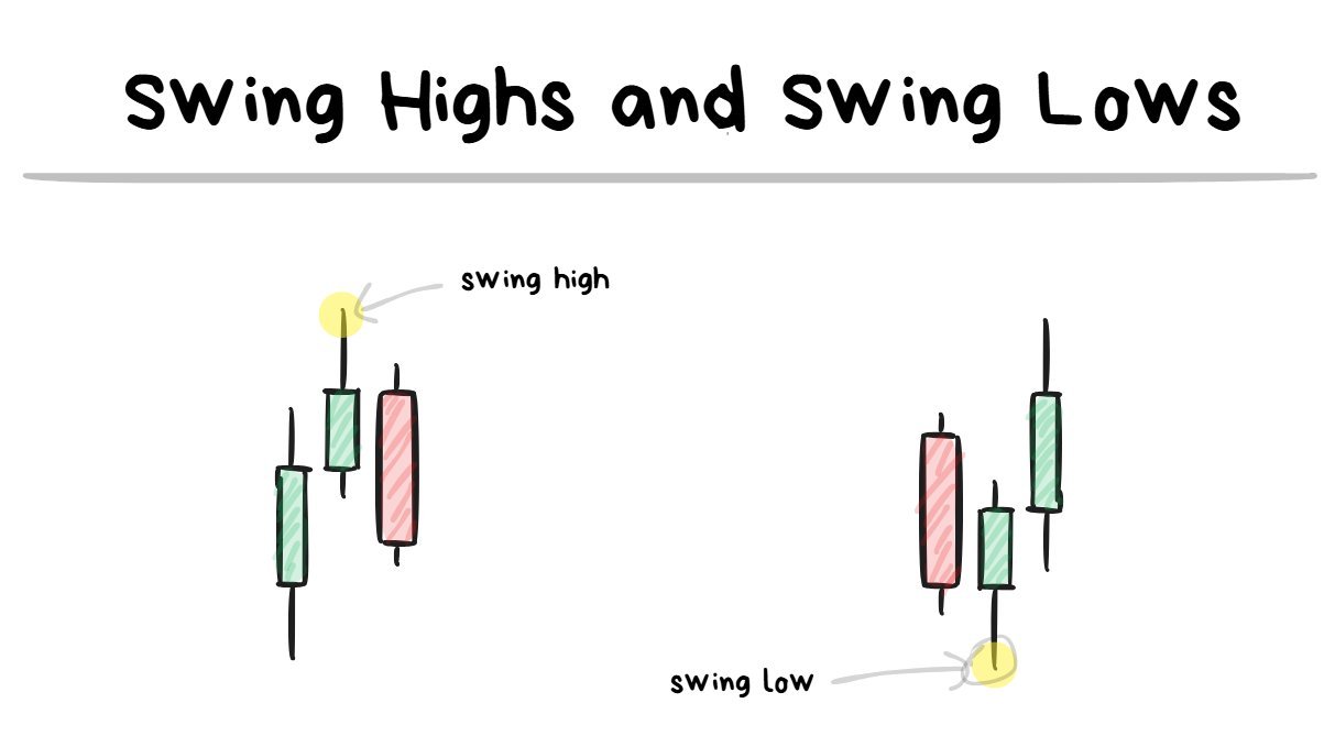
**🤓**NOTE TO READER: A swing point (high or low) requires at least 3 candles to be formed. Swing highs is when the 2nd candle has the highest extreme and a swing Low is when the 2nd candle has the lowest extreme.
These are the easiest price-action based support/resistance levels to use because of how simple it is to identify them and be consistent when using them.
I want to give some Simple Examples of using swing highs/lows below ↓
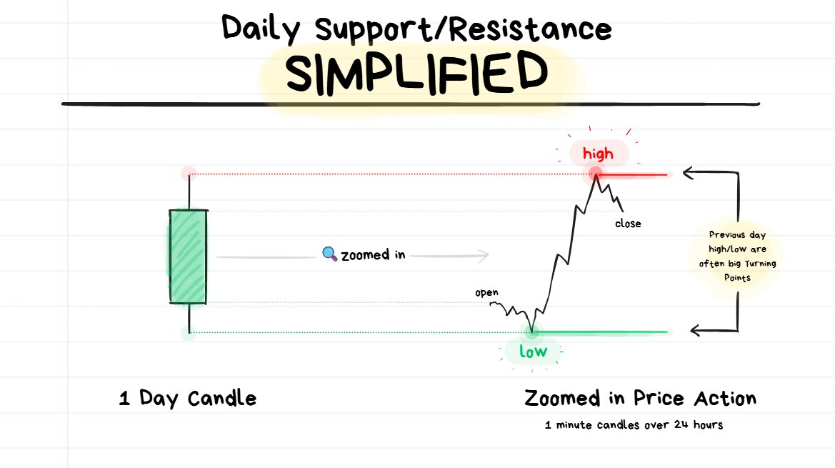
When you are looking at a 1 Day Candlestick and then you zoom into it by changing timeframes, you will get a chart which looks like something on the right hand side of the image above.
The highest and lowest points of the day often have a lot of limit orders placed near them.
A lot of market participants make their decisions based on the highest and lowest points of the day.
It is a frequent used area for traders to enter trades and also exit trades, which often causes there to be a lot of activity around these types of levels.
📚EASY EXAMPLE #1: Daily Highs/Lows
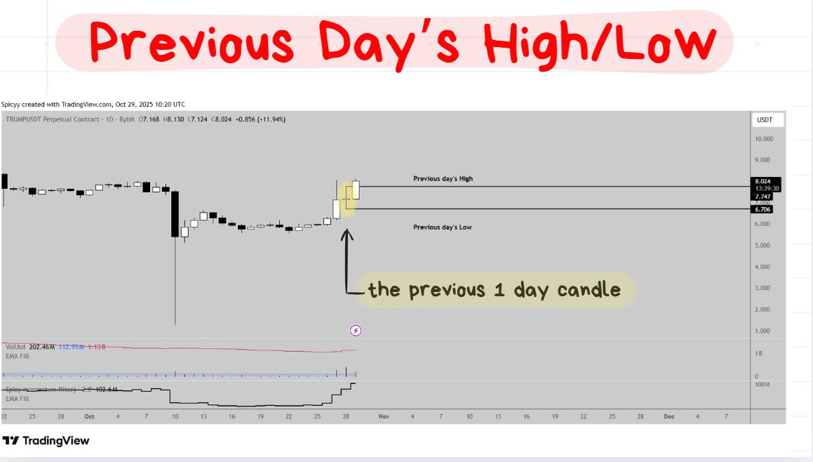
https://www.tradingview.com/x/HZgYO69I/
The Previous Day’s High/Low is one of my favorite S/R levels to trade from because of how easy it is to be consistent with execution.
When levels are drawn in the exact same type of way for every single trade, the trades become more consistent.
❗️****TIP: The High/Low of the previous X units of time will always appear as a swing high or a swing low. This is because it is only looking at the extreme points.
As executed trades become more consistent, the trades become easier to review and make improvements to.
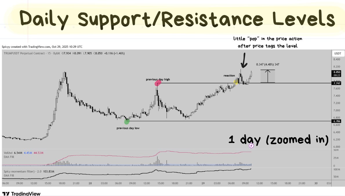
green/red dots (previous day’s high/low) were the key turning points for that 24 hours.
When you zoom into the previous day’s candle by switching to a different timeframe you’ll often be able to see how the previous day’s highs/lows were key turning points throughout the day.
When price returns to a place where a lot of volume was previously executed (which are often the key turning points), it often has a lot of volume executed there once again.
This is why we so often see more violent reactions once price reaches one of these key levels.
📚EASY EXAMPLE #2: Previous 1 Hour Swing Highs/Lows
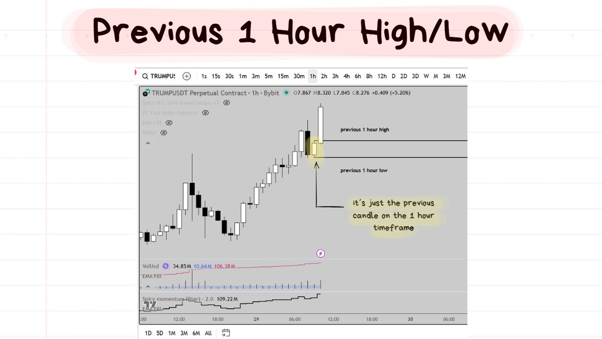
timeframe: 1 hour
Super simple:
Switch to the 1 hour timeframe.
Find the high/low of the previous 1 hour.
❗️****TIP: You can use the Magnet Tool (bottom left hand corner of tradingview) to “snap” to the highs/lows.
Then Zoom into the 1 minute timeframe. ↓
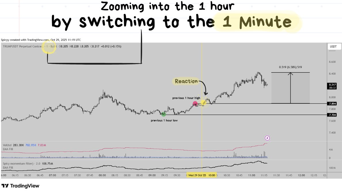
https://www.tradingview.com/x/sj72rlov/
The idea here is the same as the 1 day candles. The highest and lowest points of the previous 1 hour can often have violent reactions.
Summary: Lesson 2
Support and resistance aren’t “magical lines”. They are just clusters of limit orders.
- Core idea: Price reacts at levels where large limit orders sit. The lines we draw only visualize these areas of liquidity.
- Order size vs volatility: Bigger limit orders = bigger reactions once hit. It’s not “strong” or “weak” levels. What matters is just how much money is sitting there relative to nearby prices.
- 3 Tips: - tip1) Round numbers (e.g. $1, $10, $100) often have stacked orders. - tip2) Use tools like TapeSurf to see real limit orders on multiple exchanges. - tip3) The longer price stays away from a level, the stronger the reaction when it returns.
- Swing highs/lows: Simple, consistent S/R levels formed by 3 candles (middle one is the extreme). Daily highs/lows → high activity, great for consistency. Hourly highs/lows → good for intraday reactions.
👉 In short: Support/resistance = where real money (limit orders) sits. Trade from clear swing highs/lows and round-number levels if you want to simplify your execution and also make it more consistent.
Lesson 3: Ranging Structure and Trending Structure
Sep 2, 2025
The 2 main Trading Styles I rely on explained↓
In this lesson we’re going to cover:
- Market Structure
- Break in Market Structure
- Mean-Reverting Markets (ranging)
- Momentum Markets (trending)
- **🧠**Margin of Error (important concept)
🤓NOTE TO READER: Before diving into the lesson I want to give some quick context.
When price approaches any support/resistance level we as Traders have 3 types of decisions that we can make:
- 1 ) I bet that price will break through this level (Momentum)
- 2 ) I bet that price will bounce off this level (Mean Reversion)
- 3 ) I don’t want to bet at all. (No Trade Taken)
Before we take a trade, we have to assess multiple variables to see which of these 3 decisions is the most appropriate to make at the time.
As a Trader you have to get used to picking Option 3… a LOT.
Okay let’s get into the Lesson now ↓
Market Structure
Apr 15, 2025
Market Structure a Simple and Easy thread
Before jumping into a trade it can be quite helpful to have a little bit of context.
Looking at the current Market Structure is a good place to start.
- 🐂Bullish Market Structure: higher highs and higher lows.
- 🐻Bearish Market Structure: lower lows and lower highs.
❗️TIP: Look at the swing highs and swing lows created in the price action when trying to judge the market structure.
Break in Market Structure
Just because price currently has Bullish Structure doesn’t mean that it will just go up forever.
There are going to be times where the structure “breaks” and price can potentially turn around and start moving in another direction.
- Just because a Lower High comes in does NOT mean the structure has broken yet
- The structure is only broken when the Lower Low comes in.
- A Lower Low = the break of the most recent swing low that was formed.
- Just because a Higher Low comes in does NOT mean the structure has broken yet.
- The structure is only broken when the Higher High comes in.
- A Higher High = the breach of the most recent swing high that was formed.
Live Trade Example of using a Break of Structure ↓
Oct 17, 2025
$IP Break of structure after spiking (and almost immediately rejecting) the big $6 level. have a tight FTA on this one (lowkey am thinking that X is not the best place for posting setups… )
Mean-Reverting Markets (Ranging)
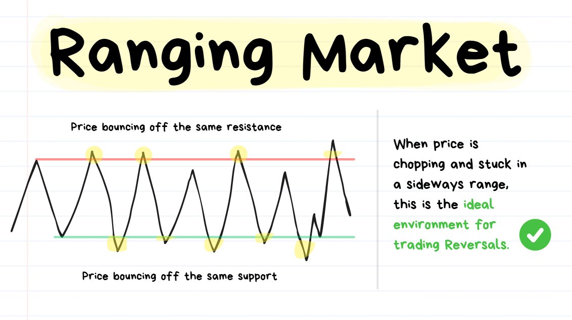
❗️****TIP: **“**Mean Reversion” means “reverting back to the mean” or “reversing back to the average/middle price.”
When the direction of price isn’t clear because it just keeps reversing from the same highs/lows over and over again, this is a Mean Reverting Environment.
This type of environment is:
- ✅the BEST for trading reversals
- ❌the WORST for trading breakouts
Momentum Markets (Trending)
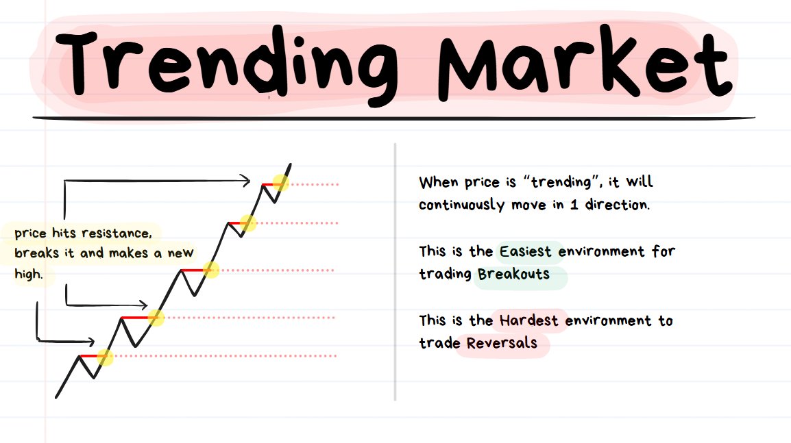
❗️****TIP: “Trending” means that price is consistently moving in 1 direction. If it’s an up trend then price is consistently going up and if it’s a down trend then price is consistently going down.
When the Market Structure of a move appears to be Bullish or Bearish for a consistently long duration of time (it’s more about total # of candles rather than units of time, since this concept holds true for all timeframes), then you’re looking at Trending Price Action.
Common characteristic of strong Trending Price Action:
- Price hits a resistance and then effortlessly breaks through it, drifting to the next resistance.
- Then when it reaches the next level, it breaks through that again and the cycle continues.
This type of environment is:
- ✅the BEST for trading breakouts
- ❌the WORST for trading reversals
🤓NOTE TO READER: This next concept had a huge impact not just on my trading but also in the overall quality of my decision-making. Of all the things discussed in this article, I hope this specific concept is the one that gets retained in your memory.
🧠 Margin of Error
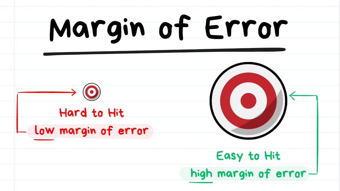
If your goal was “just hit the target”, it would make more sense to play on the 2nd Target rather than the 1st Target.
There is a reason why some environments are great for reversals and others are great for breakouts.
The reason is due to the “Margin of Error” that’s available.
- High Margin of Error = there’s a lot of breathing room for mistakes. You can make errors and still get away with it.
- Low Margin of Error = there is barely any breathing room for mistakes. You need perfect execution and even the slightest error will result in failure.
I want to quickly give the Poker analogy for this ↓
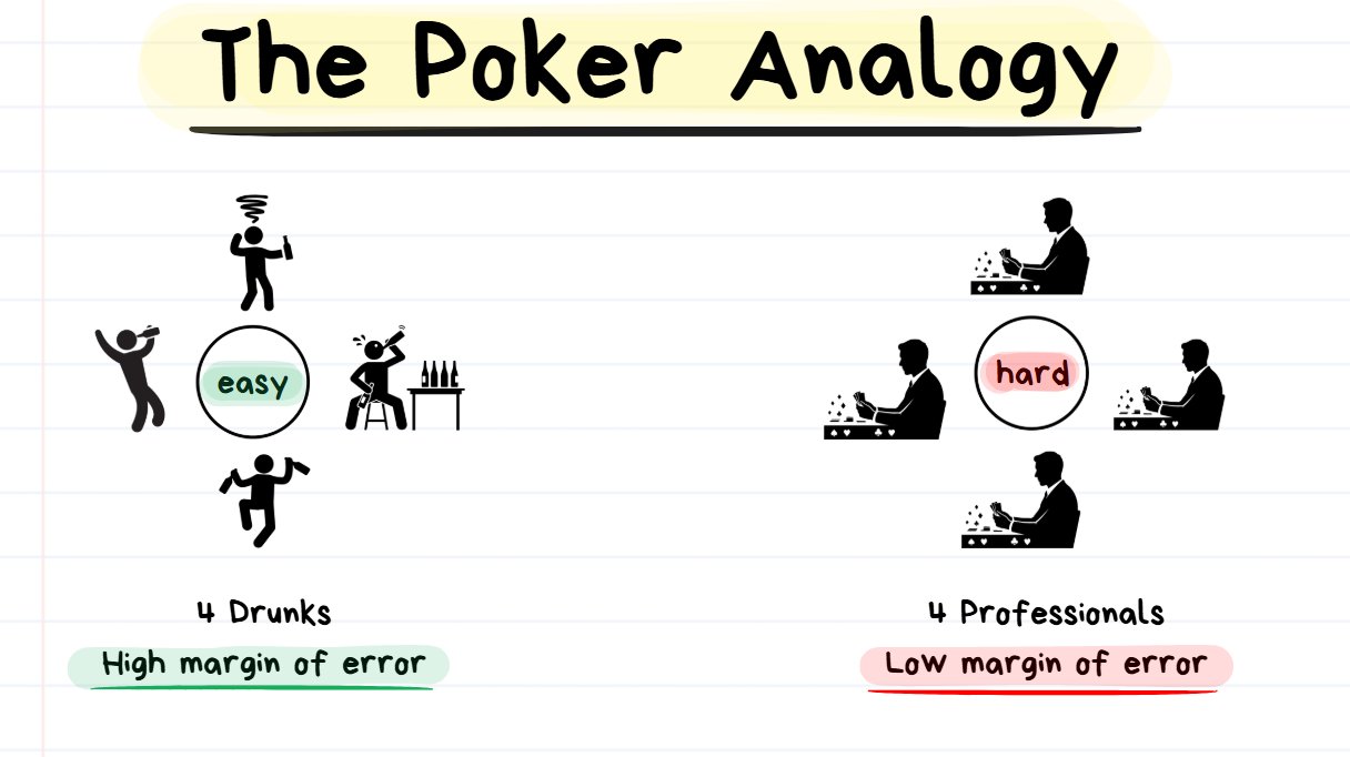
If your skill is the same but you play in an easier environment = you will have a higher earning potential.
- Saturday Night: Imagine playing Poker against 4 drunk players on a Saturday night
- Tuesday Morning: Imagine playing poker against 4 professionals on a Tuesday morning
Despite you having the exact same level of execution skill, it’s more likely that you perform better against the 4 Drunk Players rather than the 4 Professionals.
With the 4 Drunk Guys, you can make plenty of mistakes and you won’t be exploited for them. They will make plenty more errors than you, so you just have to be there to take advantage of the mistakes. Your margin of error is HIGH in this situation.
With the 4 Professionals, every mistake you make is a really big deal. You will be punished very harshly for every error and you will need to play perfectly. Your margin of error is LOW in this situation.
Imagine that BOTH situations (playing against the drunks or the pros) had the SAME PAYOUT… Then it would be a no-brainer to just only play against the drunks and to stay away from playing against pros.
🤓NOTE TO READER: Below I will explain how Margin of Error is relevant in Trading ↓
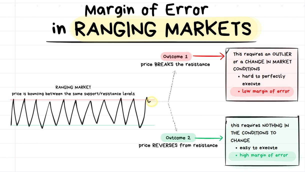
betting on Outcome #2 is easier than Outcome #1
When price is stuck in a range and then approaches a resistance level there are 2 possible things that can happen:
- OUTCOME #1: The market environment changes and price does something COMPLETELY DIFFERENT to before. The price BREAKS the level and shoots upwards. This has a low margin of error.
- OUTCOME #2: Nothing changes in the market environment. Price REVERSES from the level once again and moves down. This has a high margin of error.
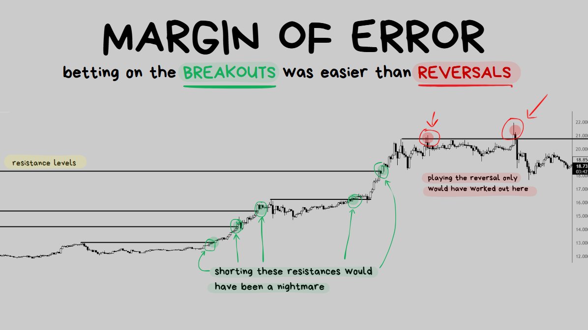
Let’s compare the margin of error with playing the reversal and playing the breakout.
🎯Timing the ENTRY:
- Reversals: Whether you played the reversal on the 1st touch of resistance, the 2nd, 3rd, 4th…. 9th…. every single one of them would have been winners.
- Breakouts: If you went for the breakout every single time that price touched the resistance, every single trade would have failed and resulted in a loss.
🎯Timing the EXIT:
- Reversals: Every single trade that was taken as a short from resistance immediately started going down. This means that it doesn’t even matter how the exit is executed, almost every single variation of taking profit would work. “Close after 10 candles” = profitable. “Close once price reaches the next support level” = profitable. “Close at the midpoint of the range” = profitable. “Close with a Trailing SL in profit” = profitable… the point is that every variation of trying to exit the trade would likely work.
- Breakouts: Since every single trade that was taken as a long from resistance immediately started going down, exiting for a profit would be insanely difficult. The only way a trade would exit in profit is if the Trader was catching the small “blip” in price as price wicked through the level and they managed to close it just perfectly in time before it turned around… but even with this method they would be catching tiny scraps. All other variations of trying to exit a Breakout Trade on the previous price action would fail and result in losses.
THE POINT ↓
As we can see, this price action gives A LOT OF ROOM for mistakes when trading reversals and VERY LITTLE ROOM for mistakes when trading breakouts.
A low quality reversal strategy would perform very well in this environment however even a highly optimized breakout strategy would really struggle in this environment.
**🤓**NOTE TO READER: The little section below with the Trending Markets might sound a bit repetitive. I just really want to emphasize the point here.
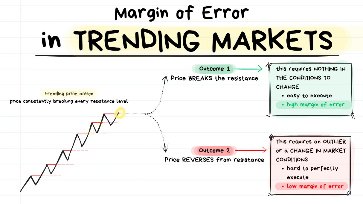
Betting on Outcome #1 is going to be easier than betting on Outcome #2.
When price is consistently trending in 1 direction and then approaches a resistance level there are 2 possible things that can happen:
- OUTCOME #1: The market environment changes and price does something COMPLETELY DIFFERENT to before. The price REVERSES from the level and falls down. This has a low margin of error.
- OUTCOME #2: Nothing changes in the market environment. Price BREAKS the level once again and continues to move upwards. This has a high margin of error.
Just like in the previous example, let’s compare the Margin of Error with both the outcomes.
**🎯**Timing the Entry:
- Breakout: If you entered earlier or later, on the 1st level or the 2nd or 3rd… it wouldn’t matter. Every single time you would have went for the breakout you would have won. The only way you would lose the trade is if the A) the conditions change or B) You get unlucky with an “outlier spike” to the downside.
- Reversals: Every single attempt at shorting the resistance would fail. The only way you could win the next attempt at shorting resistance is if you get lucky with the conditions changing in your favor or if the price randomly spikes down. It will require perfect execution since your entry will need to be based on a “change of conditions” rather than “conditions remaining the same”, which is much more challenging to do.
🎯Timing the Exit:
- Breakouts: Again here even if you were ambitious with the targets or very conservative, you would win all of the breakout trade opportunities on the left. Even if you were looking to exit with a trailing SL or something else like a MA crossover, you would likely exit with a winning trade regardless of what settings you put in your indicator or trailing SL.
- Reversals: Either you would need to go for really perfect/precise tiny winners to snipe the tiny pullbacks (which would be very dangerous and hard to do) or you will need a really clean exit if the conditions were to change. Basically shorting all of the resistances on the left hand side would be very difficult to do successfully.
Summary: Lesson 3
Every trade fits one of three decisions: 1️⃣→ Bet on a breakout (momentum). 2️⃣→ Bet on a bounce (mean reversion). 3️⃣→ Take no trade.
Your job as a Trader: identify the environment and choose the option with the highest margin of error (most room for mistakes).
1. Market Structure
- Bullish: higher highs + higher lows
- Bearish: lower lows + lower highs
- Break of structure: confirmed only when price breaches the most recent swing high/low.
2. Market Environments
A. Mean-Reverting (Ranging)
- Price repeatedly bounces between similar highs/lows.
- ✅ Best for reversals
- ❌ Worst for breakouts
B. Momentum (Trending)
- Price consistently breaks through levels and continues in one direction.
- ✅ Best for breakouts
- ❌ Worst for reversals
3. Margin of Error 🧠
- High margin of error: Easy environment, you can be imperfect and still win.
- Low margin of error: Hard environment, one mistake and you lose. Think poker: playing against drunks (easy) vs pros (hard). You want to trade where mistakes are forgiven.
4. Applying It
In ranges → reversals have high margin of error. In trends → breakouts have high margin of error. Trade with the environment, not against it.
🤓NOTE TO READER: Well done for pushing this far into the article. Just 1 final lesson to go. ↓
Lesson 4: Live Trade Examples + 5 Bonus Resources
So I’m getting really close to the image limit on this Article (yes… X articles have image limits) so unfortunately I can’t ramble on with more theory.
This final Lesson will include:
- Live Trade Examples and Explanations
- 5 Bonus Resources on Price Action related concepts
Live Trade Examples and Explanations
⚠️Quick Disclaimer: I have “cherry-picked” winning trade screenshots below. I can assure you that I do not have a 100% winrate , it’s actually sitting somewhere between 55-60%~.
🤔Quick Context: There are many influencers who say things like “you should only be shorting resistance, longing it is stupid!” Unfortunately they don’t have a clue what they’re talking about. Under specific circumstances (when margin of error is really low) shorting resistance can be a really bad idea. I want to emphasize this with 5 examples below.
Trade 1: Momentum Long
Jul 18, 2023
target hit +1.99% ty
Price was consistently breaking resistances over and over again.
The play here was “whatever was happening, I’m going to bet that nothing is going to change and it’s just going to keep happening.”
Extra Confluences:
- price action looked like a “slow grindy staircase” (good for breakouts, bad for reversals)
- the volume was increasing over time (good for breakouts, bad for reversals)
Trade #2: Momentum Long
Jul 18, 2023
first trade hit target, +1.58% ty, next please
Looks pretty much identical to the trade above:
- Slow grindy staircase price action
- Price breaking out of every visible resistance on the left hand side
- Consistently increasing volume over time
This is a perfect example of “would rather be long until I’m wrong rather than short until I’m right.”
All Traders who were furiously shorting every resistance were not having a fun time during this trend.
Trade #3: Momentum Long
Jun 22, 2023
target hit +5.6% next please
This one is a bit more of a “steeper” and “more extreme” example, but the concept remains the same.
- The market structure was bullish (higher highs and higher lows)
- Price kept slicing through every resistance like a hot knife going through butter
- Volume was consistently increasing over time
Margin of error for breakout trading was very high but for reversals it was very low.
Even if I botched the entry and mistimed the exit the market would have rewarded me… but for trading the reversal I would need absolute perfect and very precise execution.
Trade #4: Momentum Long
Jul 10, 2023
target hit +6.7% tyvm
You must be tired of seeing the exact same price action, same thing in volume, same behavior of price exploding through every visible resistance…
… if yes, then get used to it because this is how consistent execution feels like.
Taking the exact same trade in the same conditions with similar outcomes over and over again.
I’m trying to drill the repetition here to show that these specific scenarios are generally VERY UNFAVORABLE for going for the reversal trade which inversely makes it VERY FAVORABLE to attempt going for the breakout instead.
Trade #5: Momentum Long
Jun 4, 2023
Target hit +1.59% onto the next
Same exact thing. Margin of error is really high on this one.
- I could have entered a few candles earlier, a few candles later…
- I could have exited a little bit earlier or a little bit later
- I could have used a slightly different timeframe
- .. and most of the variations of how this trade could have possibly been taken likely would have ended up as a winner.
Staircase-like price action (cleanly breaking through every resistance) on increasing volume is REALLY NICE for trading breakouts and I will continue to repeat it over and over again.
🤓NOTE TO READER: Hopefully my words and this price action pattern gets tattooed into your memory.
5 Bonus Resources on Price Action
Below I’m going to dump 5 Bonus resources/materials which you may find helpful.
Enjoy! ↓
1. How I trade Breakouts
Jul 31, 2025
2. How I trade Reversals
Oct 1, 2025
3. How I use Crypto Screeners to make it easier to tell if I should be focusing on Breakouts or Reversals
Oct 14, 2025
4. Volume Masterclass
Oct 23, 2025
5. Thread on Price-Action Confirmations
Oct 14, 2025
Trade Entry “Confirmations” I notice traders regularly asking questions about this topic Here’s a small Thread of some Resources: (1/4)
Article Summary
Lesson 1: How Price Actually Moves
- Price moves because of supply and demand, not secret algorithms.
- Makers = limit orders that add liquidity.
- Takers = market orders that consume liquidity.
- When market orders eat through the limit orders at one price, price shifts to the next.
- In short: 👉 Price = the result of market orders hitting the orderbook.
Lesson 2: Support & Resistance
- S/R levels aren’t magical lines, they’re zones where clusters of limit orders sit.
- Price reacts violently when big limit orders are hit.
- It’s not about “strong” or “weak” levels; it’s about how much money is sitting there.
- Round numbers and previous highs/lows attract heavy order flow.
- Key setups: Daily highs/lows = consistent and reactive. 1-hour highs/lows = great for intraday trades.
- 👉 Focus on liquidity clusters, not artistic lines.
Lesson 3: Ranging vs Trending Structure
- Every trade decision = 1️⃣ Bet on a breakout (momentum) 2️⃣ Bet on a bounce (mean reversion) 3️⃣ Don’t trade
- Bullish structure = higher highs/lows. Bearish structure = lower highs/lows. A break in structure = breach of the last swing high/low.
- Ranging markets: best for reversals, worst for breakouts.
- Trending markets: best for breakouts, worst for reversals.
🧠 Margin of Error Concept
- Some environments forgive mistakes; others punish them.
- High margin of error = easy to win even with sloppy execution.
- Low margin of error = need perfect timing.
- Like poker: trading against drunk players (forgiving) vs pros (punishing).
- In ranges → reversals have higher margin of error.
- In trends → breakouts have higher margin of error. 👉 Trade where mistakes are forgiven, not where precision is mandatory.
Lesson 4: Live Trade Examples + 5 Bonus Resources
- Real trades illustrate repetition and consistency: “Same setup, same behavior, same outcome.”
- Breakout longs during trending markets show: Staircase price action. Increasing volume. High margin of error = even imperfect entries/exits work.
- The point: You make consistent money by repeatedly executing the same high-probability setups in forgiving environments.
I am very grateful to you for giving me your Time and Attention, your 2 most valuable assets.

🌶️
Source
Written by @spicyofc · View original post · Published: 2025-09-02
Risk Management Guide for Traders
There are many important things to manage, but nothing is as important as Risk.
I’m a former Prop Trader and I’ve been trading Crypto for 8 Years.
First I want to say thank you for taking time out of your day to click on this article and give it a read. Your time and attention are very valuable resources, so I am grateful for you to give some of it to me.
In exchange, I will give you everything I know about Risk Management.
I have done my best to simplify everything in here for you.
✍️ Let’s get started ↓
Overview
- Lesson 1 ) The Expected Value (EV) Equation
- Lesson 2 ) The Monte Carlo Simulation
- Lesson 3 ) What is Leverage and Liquidation
- Lesson 4 ) The difference between “Position Size” and “Risk”
- Lesson 5 ) Risk of Ruin + Good Bet Sizing
Lesson 1: The Expected Value (EV) Equation
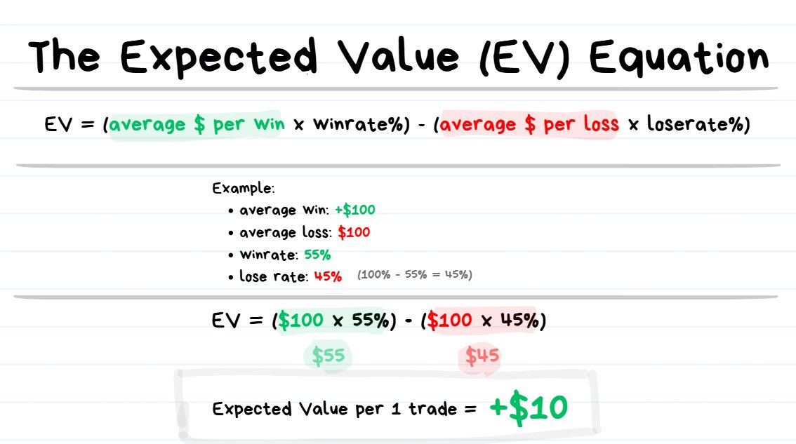
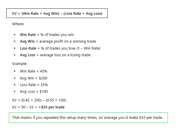
EV= (Average Win x Win%) − (Average Loss x Loss%)
❗️TIP: Expected Value = the average outcome you can expect if you repeated the same decision over and over.
Every single Trader NEEDS to know what Expected Value is and how to calculate it.
🤔Why is EV so important?
- The Expected Value of a Trade allows us to estimate what our expected profit will be over the next N number of trades.
In the image example I shared above, if you have an expected value of +$10 per trade, then if you take 1000 of this exact same trade then your average “expected profit” should be roughly $10 x 1000 = $10,000.
- If you have a POSITIVE EXPECTED VALUE (+EV) , your trades will win money over time.
- If you have a NEGATIVE EXPECTED VALUE (-EV), your trades will lose money over time.
In the section below I will talk about the Monte Carlo Simulation which helps visualize this. ↓
Lesson 2: The Monte Carlo Simulation
In this Lesson I’m going to cover a few things:
- The Monte Carlo Simulation
- Variance
- The Law of Large Numbers
- How these 3 things above related to Trading
This might look scary because of numbers, fancy names and graphs, but I promise it’s fairly simple to understand.
I believe having a basic understanding of these 3 topics will make everything to do with Risk Management easier to digest.
First let’s quickly cover the Monte Carlo Simulation ↓
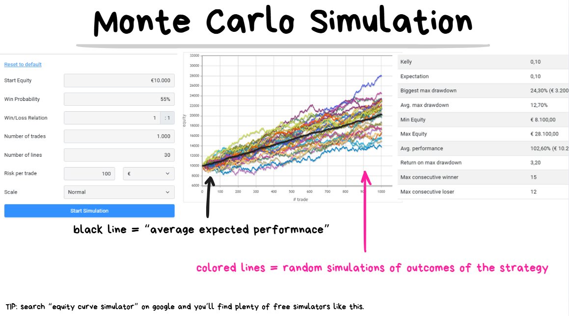
30 simulations of how performance can look like with a 55% winrate, 1R strategy over the next 1000 trades. This is a profitable (+EV) strategy.
❗️TIP: Monte Carlo simulation = running lots of random “what if” scenarios to see all the possible outcomes after taking N number of trades.
A Monte Carlo Simulation can help us manage expectations and also give us a rough idea for how profitable our strategy is.
We input our starting balance, winrate %, average win/loss ratio and the # of trades, and the simulation will spit out random combinations for how our performance can look like.
The thick black line visualizes the “average expected outcome”.
So if our EV per trade is +$10 and we take 100 trades, our total profit will be “roughly” +$1000~ . If we take 1000 trades with the same strategy then our total profit will be “roughly” +$10,000.
Notice the emphasis on the word “roughly”. This is because it cannot be guaranteed and there can be a bit of variance.
Secondly, let’s quickly talk about Variance ↓
“Randomness” plays a role in our trading performance, whether we like it or not.
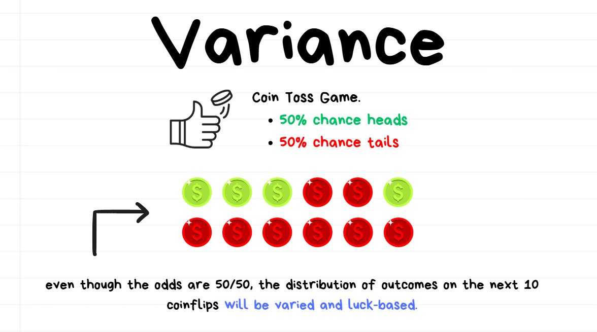
🧠Here is a Coin Flip analogy
- Imagine you are playing a Coin Toss game with a 50% chance of getting either heads or tails.
- If you flip the coin 10 times, it is possible to get heads 8 times and tails 2 times. Despite the chance of landing on heads is 50%, it landed on heads 80% of the time.
- This DOES NOT mean that the coin is rigged and has a 80% chance of landing on heads.
- It just simply means that the coin has not been flipped enough times for the probabilities to properly play out.
- The difference between “actual outcome” (80%) and “probability” (50%) is the variance (80% - 50% = 30%)
- If you were to flip the coin 10,000 times, you might get 5050 heads and 4950 tails. Even though the the raw difference is +50 more heads than expected, in percentage terms there is only 0.5% (50 ÷ 10000) of variance.
Thirdly, let’s quickly discuss The Law of Large Numbers ↓
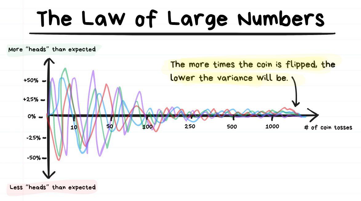
The more times that a coin is tossed, the closer the Variance gets to 0.
❗️TIP: The “Law of large numbers” means the more times you repeat something random, the closer your results get to the true average.
If you play the coin toss game only 10 times, there is going to be a lot of variance in the % of times that the coin landed on heads.
If you play the coin toss game 10,000+ times, there is going to be very little variance in the % of times that the coin landed on heads.
Basically the more you times an event happens, the closer the outcomes will start to move towards the “real probability”.
How does a Monte Carlo Simulation, Variance and Law of Large numbers all relate to Trading?
The Monte Carlo Simulation allows us to manage our expectations (baed on the variance) over how our next N number of trades are going to play out. The more trades taken, the less variance we can expect.
- How much expected profit should we see after N trades?
- How many consecutive wins we can expect to see?
- How many consecutive losses can we expect to see?
- How much of our account is it “normal” to lose with this kind of winrate and risk/reward ratio after N trades?
It’s also a “slap-in-the-face” reality check about certain truths:
- Even highly profitable strategies can go through extended periods of drawdown. (Drawdown = how much % have you lost in the account)
- Even high win-rate strategies can go on large consecutive lose streaks.
- Even terrible, low win-rate strategies can go on large consecutive win streaks.
- The outcome of the next trade we take DOES NOT MATTER. What matters is the outcome of the next 100+ trades we take.
The Main Takeaway
→ Sometimes you’ll make a good trade and lose.
→ Sometimes you’ll make a bad trade and win.
It’s going to happen because of variance/luck.
Judging whether or not you made the good trade based on 1 outcome is not the way to go.
Two Extreme Examples ↓:
- You take a trade based on a pattern which has a 90% success rate with a Risk/Reward ratio of 1: If you take the trade and it loses, it was still the right call. This is because if you were take the same trade 1000+ times and let the law of large numbers play out, you would be printing money. ✅
- Playing at a Slot Machine in a Casino: If you win once, that doesn’t make it a smart bet. You just got lucky due to variance. If you keep betting 1000+ times and let the law of large numbers play out, then you would get wiped out for all of your funds. ❌
The point: Don’t judge your trade quality based on whether the next trade is a win/loss. Instead judge them by their expectancy. You will need to be patient and sit through some variance before the profits start rolling in.
Lesson 3: What Is Leverage and Liquidation?
Leverage is probably one of the most misunderstood concepts for Traders.
🤓QUICK NOTE TO READER: Before reading everything below I want to make it clear that you DO NOT have to remember every single thing below, so don’t stress.
As long as you get a “basic understanding” of what leverage is, you’ll be fine.
👨🎓 Mini Test: Do You Understand Leverage?
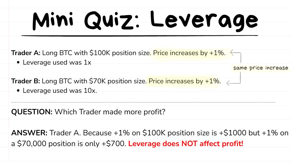
(assume the entry price of both traders is the same)
What most people think Leverage is (but it is DEFINITELY NOT this ❌):
- A turbo profit multiplier, such when you slide it up it magically increases how much money you’re going to make on the trade.
- I promise you, leverage is NOT this.
What Leverage ACTUALLY is ✅****:
- A tool to reduce counterparty risk and also improve capital efficiency.
- Counterparty Risk = the funds that you risk by holding on an exchange. It is at risk because there is non-zero chance of the exchange rugging/scamming (e.g. FTX).
- Capital Efficiency = how efficiently you can use your money to generate more money. For Example: Needing $1000 of capital to make $1000/month is 100x more efficient than needing $100,000 of capital to make $1000/month.
🤓Before going further, let’s first get some clear definitions on some terms. Then we can return to learning more about Leverage. ↓
- Trading Account Balance: the total capital you are willing to use to execute trades.
- Exchange Account Balance: the amount of money you have deposited onto the exchange. This is naturally going to be a small % of what your entire trading account is. It is not recommended to have your all 100% of your entire trading account deposited onto an exchange.
- Margin: The required money that you need to put up in order to open a trade.
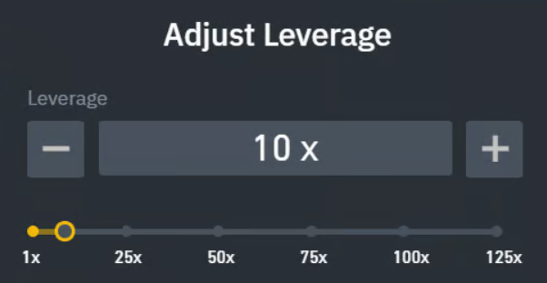
- Leverage: The multiplier of the money that you are borrowing from the exchange.
- Position Size: The total amount of whatever coin that you opened a trade in.
🤓NOTE TO READER: below is a post which shows a flow chart for how I manage deposits/withdrawals from exchanges. The point is to never be “over-exposed” on 1 exchange.
Aug 31, 2025
Serious Traders don’t keep 100% of their funds on an exchange. Leverage is a gift which allows using trading capital without needing to deposit it. Below is the system I use for topping up and withdrawing profits from CEX exchanges as an Altcoin Perp scalper ↓
Example: Leverage in Practice
Pretend you have $10,000 that you are willing to trade with. This is your Trading Account Balance.
You don’t want to deposit all $10,000 onto an exchange because what if the exchange decides to hold our funds, scam/rug or it gets hacked. So instead you deposit 10% of these funds onto the exchange. So $1000 gets deposited onto the exchange. Your Exchange Account Balance is now $1000.
You see a good trade opportunity in BTC and you want to long $10,000 worth of it. If you try to click “Buy”, it will say insufficient funds. Since you only have $1000 in your Exchange Account Balance, you will need to use Leverage to get the required funds to open the position.
- So you put the Leverage to 10x and then you try again and it works.
- Your Position Size (how much of the coin did you actually buy) on the Trade is $10,000.
- Your Margin (how much money did you need to put up “as collateral”) is $1000.
- Your Leverage is 10x.
❗️TIP: The profit on a $10,000 position with 1x leverage or 100x leverage is going to be exactly the same. A $10,000 position will always just be a $10,000 position. You can change the leverage of a trade literally while in the trade, and it won’t do anything to the profit.
The Purpose of Liquidation
When you are getting leverage on a position, you are basically “borrowing” from the exchange. The money isn’t magically coming out of thin air 😂.
If you open a $10,000 position using 10x leverage with only $1000 deposited on your trading account, that $9000 is lent to you by the exchange. Those “borrowed funds” can only be used for opening positions.
In order to ensure the exchange gets their lent money back, they have the Liquidation Function.
⚠️Liquidation: If price hits a certain point (the liquidation price), the exchange will forcefully close you out of your position and collect your margin (the collateral you put up). Then the exchange will be taking over your position instead and the trade will be their problem now.
I want to use an Analogy to make this easier to understand ↓
Let’s pretend that I am bullish on a new iPhone.
The price of this iPhone is $1000. I have a feeling that it’s going to go to $1100 (+10% increase in price).
My idea is I want to try to buy the iPhone for $1000 and then re-sell it for $1100, making a +$100 profit on my trade.
The only problem is that I’ve only got $100 in my bank account.
So I go to Timmy, who is a wealthy individual, and explain to him that I really want to borrow $900 so I can take this bet on the iPhone.

My beautiful MS Paint Artwork: Me asking for a $900 loan from Timmy.
Here is the issue:
- If Timmy lends me the $900 and then the iPhone drops below $900 in value, even if I re-sell it I won’t be able to pay Timmy back in full.
- Timmy will lose money for no reason. Timmy doesn’t like losing money for no reason.
Here’s the solution:
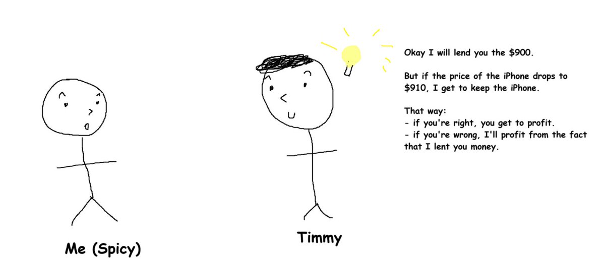
An agreement which benefits both parties is created. (Perpetual Futures Contracts are “Contracts” that are made between the Trader and the Exchange)
- Me and Timmy get a contract made together.
- If the price of the iPhone DROPS BELOW $910, I will have to give Timmy the iPhone that I bought. This is my “position being liquidated”.
- So I will lose the initial $100 that I had (the margin)
- And Timmy will try to sell the iPhone himself. If the price of the iPhone doesn’t move that much and he manages to successfully sell it above $900 , then Timmy will make a profit.
- The reason why Timmy gets to keep the iPhone if it drops below $910, rather than $900, is because Timmy deserves to get some profits for the fact that he lent me some money in the first place.
In Summary
- Traders use leverage to open positions that they want to speculate on.
- The exchange temporarily lends them the “leftover funds” that they need to open the large position.
- If the Value of the position drops below a certain price, the trader gets fully closed out and the position gets transferred over to the exchange.
- The exchange now has to try to get rid of the position.
- The exchange has a very high likelihood from profiting off a liquidation, since the “liquidation price” is always going to be favored for the exchange to give them plenty of breathing room to get rid of the position for a profit.
The Main Takeaway
You don’t have to remember what all of the terms mean.
The most important thing that you need to understand is that leverage is just a tool to help you get the position size that you need.
Also, never ever ever risk getting liquidated. The costs/fees with getting liquidated are absolutely enormous.
❗️****TIP: Always use a stoploss for every trade. It’s incredibly dangerous to trade without one.
Lesson 4: Position Size vs. Risk
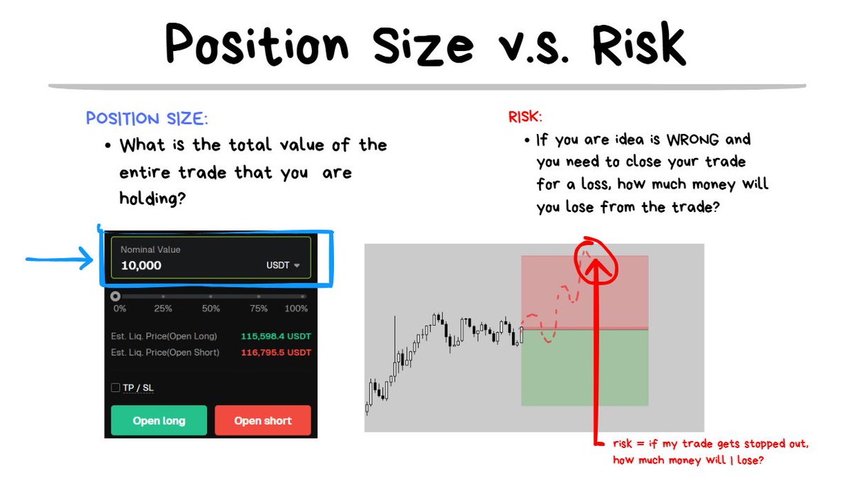
Another topic that is often misunderstood by traders is the difference between Position Size and Risk.
❗️TIP: Position Size = the total number of coins (or the USD value of the coins) that the trade is worth. (e.g. “I bought $10,000 worth of BTC. So position size is $10,000”)
❗️TIP: Risk = the amount of money you will lose if your trade idea is wrong and you need to cut it for a loss. (e.g. “If price hits my stoploss I will lose $100. So my risk = $100”)
Before I take any trade, the first question I ask is “if my idea is wrong and I have to cut my losses, how much of a loss would I be willing to take?”
This is a critical question to ask that a lot of traders completely ignore because they’re so blinded by the concept that it would be impossible for them to be wrong because their trade idea is so genius. Put FOMO into the mix and it can get nasty.
After coming up with an appropriate number to risk on the next trade, the next step is to calculate the position size.
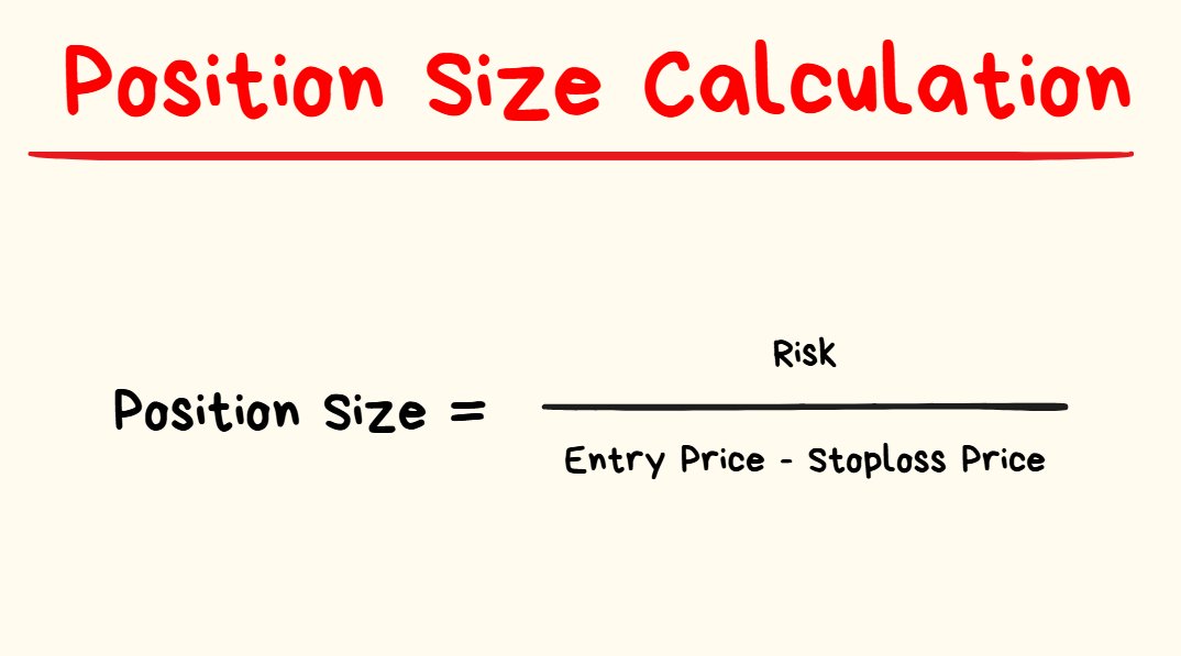
Before you panic and assume you have to “do math” before you enter every single trade, relax…
… there is an easy way to calculate it.
TradingView has the calculation built into their Risk:Reward tools ↓
Sep 21, 2025
Easiest way to calculate your Position Size relative to Risk in a Trade ↓
If you follow the 3 steps above, you’ll be able to easily see exactly how much position size you need on a trade after you just type in however much risk you want to take.
Easy peasy. Onto the final lesson 🤓
Lesson 5: Risk of Ruin + Bet Sizing
A universal Question that all traders end up asking at some point: “How much risk is the best amount of risk to take on my trades?”
The Answer: it depends. 🤷♂️
Popular Answer (which I think is a good answer by the way): Very popular advice is starting off with risking 1%~ of trading capital per trade. Meaning if you have $10,000, if you lose your next trade expect to lose -$100.
My Personal Answer: The higher the quality of the trade, bet more. The lower the quality of the trade, bet less.
Risk of Ruin + The Kelly Criterion
Let’s talk about Risk of Ruin first. 👀
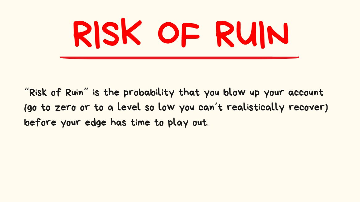
Just because you have an edge (a +EV, profitable strategy) doesn’t mean that you can’t blow up.
❗️****TIP: Rule #1 of trading is “never blow up”. If you blow up, you can’t play anymore. The whole point is to stay in the game for as long as possible.
In fact, all your chances of profitability get completely thrown out the window if you’re risking too much per 1 single bet.
Let’s use an extreme example:
- Pretend risking 100% of your Portfolio on every trade, on a strategy which has a 90% winrate with a risk:reward ratio of 10:1.
- This type of strategy is INSANELY GOOD, but the problem is if you’re going all-in every single time you are guaranteed to get wiped out eventually.
If you get wiped out, it’s game over. Even if you get “close” to being wiped out, recovering can be really really hard.
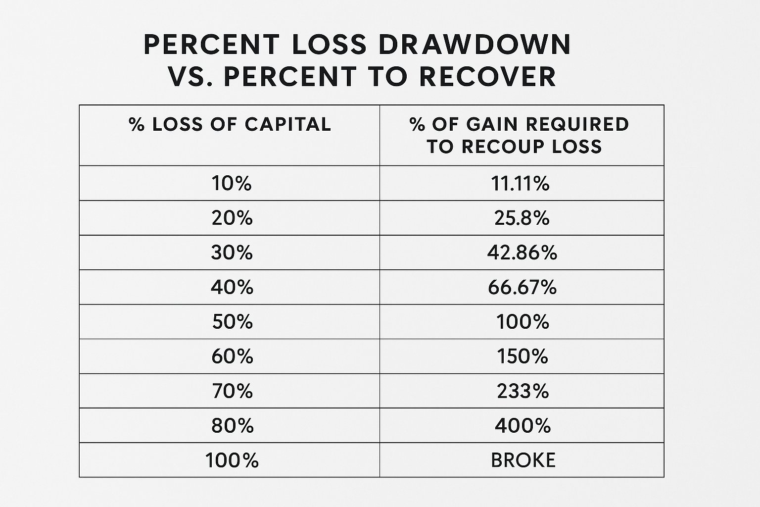
This is why growing an account feels so hard, but blowing an account feels effortless
Okay so now it should be clear that there is definitely a limit with risking too much. If we bet too big, we will blow up our account sooner or later even if we are using a good trading strategy.
But on the other hand if we risk too little, like 0.0000001% on the trade, we’re going to be little fairies who never actually end up growing an account.
So Where Is the Sweet Spot?
Let’s now talk about the Kelly Criterion, which tries to solve the riddle for the “sweet spot”. 👀
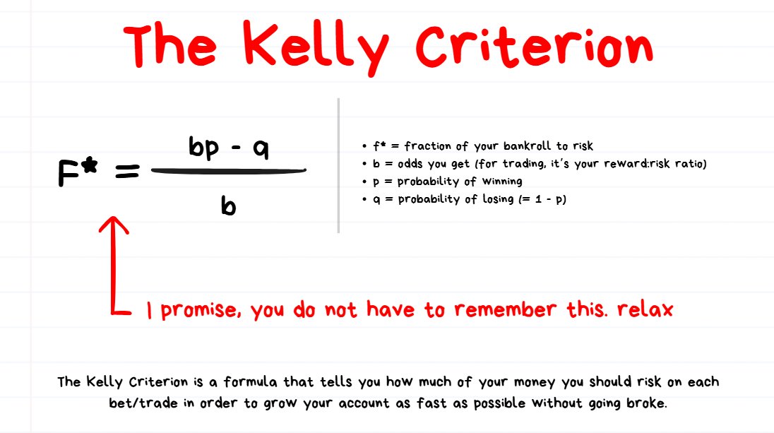
I promise, you do NOT need to remember this. I just included this for the nerds.
- Some Traders argue and say Kelly is the best approach for measuring optimal bet sizing.
- Other Traders say that it’s too conservative and slow for growth and instead take an approach to doing several multiplies of the Kelly (example: Their bet size = Kelly multiplied by 2)
- Other Traders say Kelly is still too aggressive and doesn’t take “unexpected margin of error” into account and bet even lower (example: Their bet size = Kelly divided by 2)
The Point About Kelly and Optimal Bet Sizing
- I don’t believe there is “perfect/flawless” approach to sizing your bets.
- Even if you use the Kelly or some other nerdy calculation to size your bets, nothing is perfect in the realm of trading.
As I mentioned a bit further up above, I prefer to take a “Dynamic” approach to bet sizing.
- Low Quality Trade = I don’t even bother trading these.
- Standard Quality Trade = I risk 1% on the trade.
- High Quality Trade = I risk 2% on the trade.
- Super High Quality Trade = I risk a maximum of 4% on the trade.
🤓NOTE TO READER: Is this the best approach to sizing? I have no idea! But I like to keep things simple and this approach has worked well for me.
How I measure the quality of a trade will be based on the strategy that is being used to execute it + what variables are present right before I enter the trade.
I go a lot more in-depth with “measuring trade quality” in 2 other articles that I posted.
The first one is everything with how I trade Breakouts and the other is everything to do with how I trade Reversals. You’re welcome to check them out below if you would like ↓
Jul 31, 2025
Oct 1, 2025
Summary of the 5 Lessons
- Lesson 1: Knowing the numbers behind your edge is important. Expectancy is a critical topic to understand in any “probability-based” type games such as Trading.
- Lesson 2: Remember to think about the next 100 trades and let go of the outcome of the next 1 trade. Let the law of large numbers play out.
- Lesson 3: Leverage is not a profit multiplier, it’s just a capital efficiency tool. Remember to never risk getting liquidated.
- Lesson 4: Position Size is how much of the coin you’re buying while Risk is how much money you’re going to lose if your idea is wrong.
- Lesson 5: Drawdown is naturally harder to get into than it is to climb out of. Size your bets appropriately. If you’re new, keep it simple and stick to the standard 1% per trade until getting a better understanding of your “high quality A+ trade setups”
Once again, I thank you for taking the time for pushing through this lengthy article.
If you made it this far, don’t be shy to ask questions on any topics that you want more information on in the comments.
I’ll reply to literally every single one.
🌶️
Source
Written by @spicyofc · View original post · Published: 2025-08-31
Momentum Trading Strategy
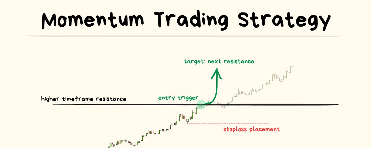
Many traders think it’s “Wrong” to make money by Longing Resistance or Shorting Support.
I’m a former Prop Trader and I’ve been trading crypto for 8 years.
I’m going to explain how I bet against reversal traders and win.
This style of trading is my niche.
Overview
- Market Conditions > Entry Rules
- Momentum and Mean Reversion
- Worst Mean Reversion Conditions
- My Momentum Trade Criteria
I will cover some concepts first and then get into the technical stuff at the very end.
It’s All About Market Conditions
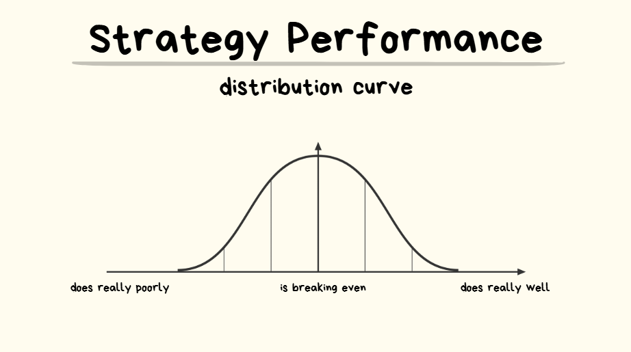
If you take 1000+ trades on any strategy there are going to be good times, bad times and “meh” times.
The first thing to understand is that ALL strategies will go through windows of time where they:
- Do really well
- Do well
- Breakeven
- Do poorly
- Do really poorly
We want less trades on the left, more on the right.
To achieve this we need to be trading more in “good conditions” and less in “bad conditions”.
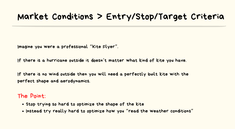
“Kite Flying” analogy
If the above is understood, it means that:
Optimizing how to define Market Conditions is actually more important than optimizing Entry/Stop/Target rules.
Momentum vs. Mean Reversion
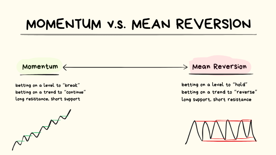
Momentum (also known as “trend following”) and Mean Reversion (also known as “reversal”)
Most strategies fall under 2 main styles:
Momentum
- buy high, sell higher
Mean Reversion
- buy low, sell high
Worst Conditions for Mean Reversion (= Best for Momentum)
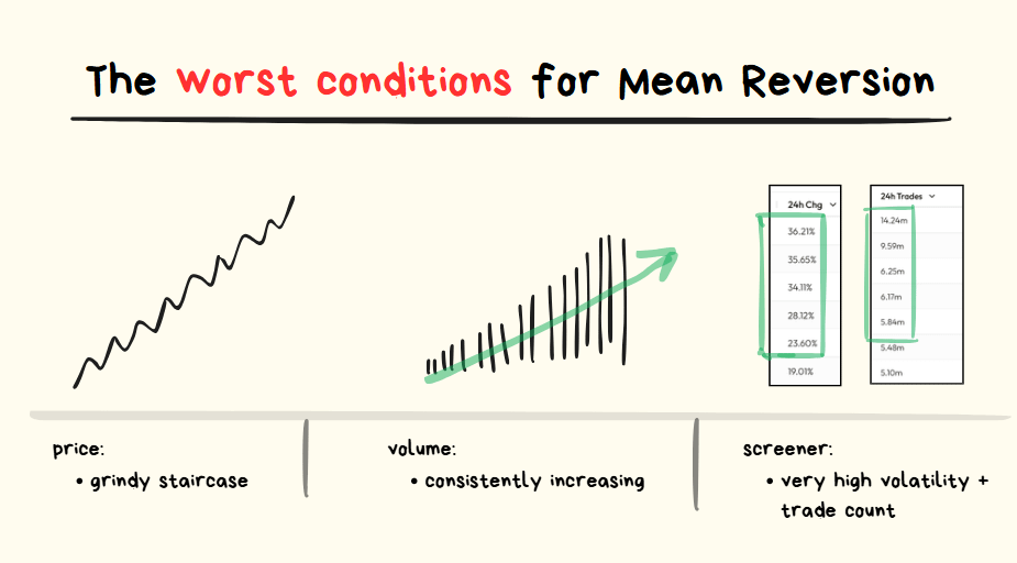
1. “grind” into the level
2. increasing volume over time
3. “staircase” type of price action
4. high volume/volatility on screener
If these are present, the coin is likely in a strong trend.
In order for us to Win we need our Counterparty to Lose.
We need to be trading when our counterparty is trading in their Hardest environment to maximize our chance of winning.
- Easy for them = Hard for us. ❌
- Hard for them = Easy for us. ✅
Live Example
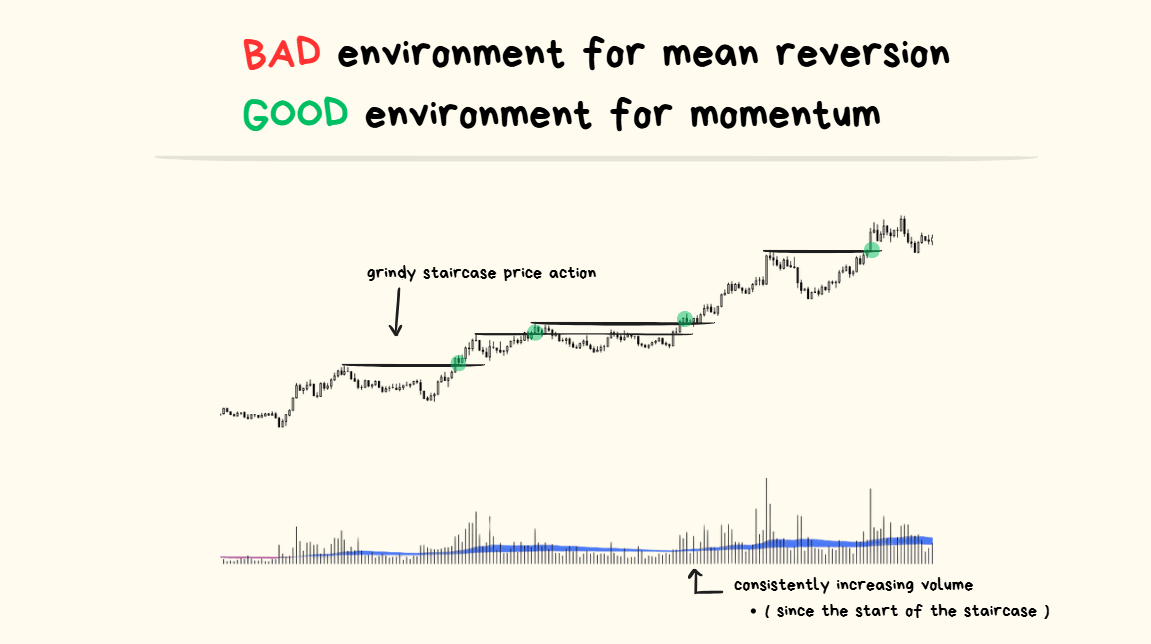
coin: ENA/USDT
date: Friday, 25th July 2025
time: 02:00 - 11:00 (UTC)
price was slicing through every resistance:
- makes it harder to short the highs
- makes it easier to long the highs
An ideal environment for taking a Momentum Long.
Momentum Trade Criteria
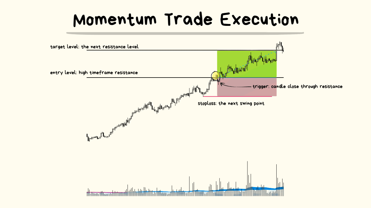
slow grind into the level ✅
volume consistently increasing ✅
staircase price action ✅
Level Selection:
- major highs/lows
Entry:
- candle close through the level
Stoploss Placement:
- 1st or 2nd swing point (both are valid)
When NOT to Take the Momentum Trade
Knowing when to step on the brakes is just as important as knowing when to step on the gas.
The #1 most important thing to avoid:
- Vertical Fast Spikes into the entry level
- These are really good for Mean Reversion, which makes it really bad for Momentum.
Example below ↓
Jul 22, 2025
fast spike reversals: these often come back to where they came from example: ↓
Summary
Longing resistance and shorting support can work really well in the right environment.
Top 3 things I look for:
- a grind into the level
- consistently increasing volume
- “staircase” price action before the entry (ideally at least 2 hours of it non-stop)
Top 3 things I avoid:
- fast/vertical spikes into my entry level
- decreasing volume
- choppy/sideways type of price action
Enjoy the Alpha 🤝

your stoploss is my target
Source
Written by @spicyofc · View original post · Published: 2025-07-22
Mean-Reversion Trading Strategy
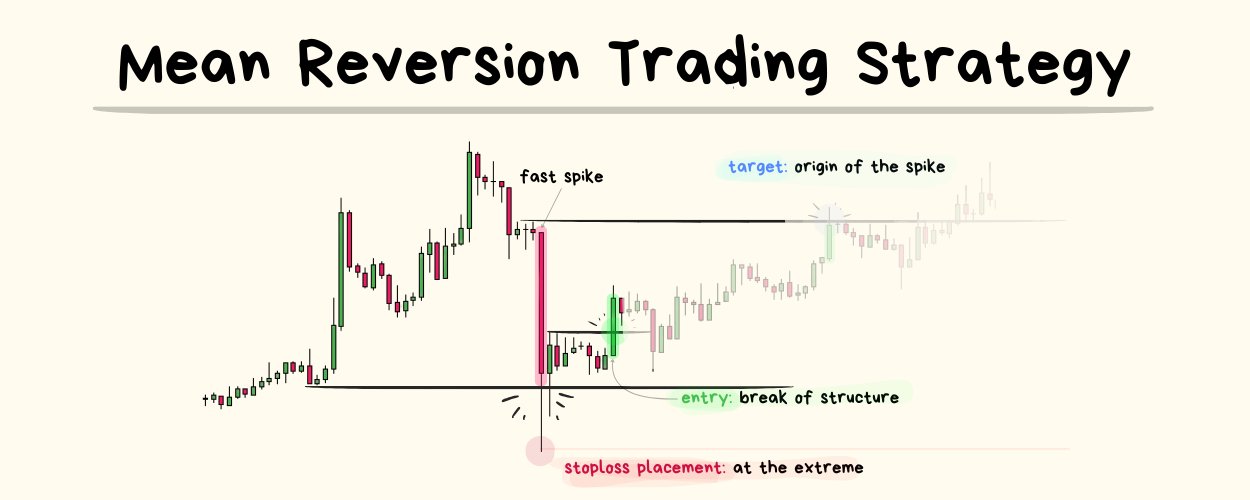
Every Trader has felt the pain of buying a dip but it just keeps on dipping.
I’m a former Prop Trader and I’ve been trading Crypto for 8 years.
I will explain exactly how I trade reversals on the 1 minute timeframe and everything I think about to avoid “buying the dips which just keep on dipping”.
Overview
Firstly I want to say thank you for clicking on this article and taking your time to read it.
Your time and attention is a valuable resource, so I am grateful that you are giving it to me by reading through this article.
In exchange for what you have given me, I hope to give you 7 Lessons that I wish I learnt earlier when learning to trade Reversals ↓
- Lesson 1 ) The 2 main Trading Styles (momentum and mean reversion)
- Lesson 2 ) My Best/Worst Trading Conditions for trading Reversals
- Lesson 3 ) How I do a “Market Scan” to check if conditions are good for trading Reversals
- Lesson 4 ) Which Support/Resistance levels I like to trade at + Setting Alerts
- Lesson 5 ) My logic for the Entry/Stoploss/Target rules
- Lesson 6 ) How I determine the quality of a Trade (low/medium/high)
- Lesson 7 ) How I cut losing trades before they hit the stoploss
✍️ Let’s begin. ↓
Lesson 1: The 2 Main Trading Styles
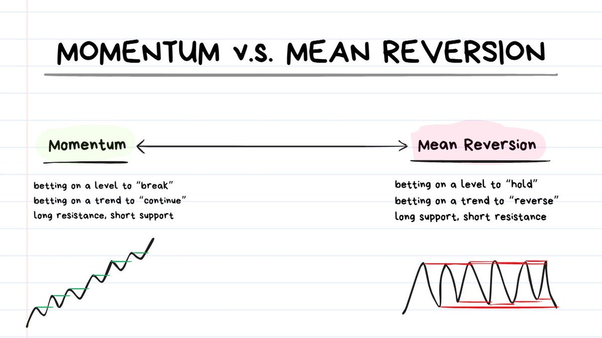
Momentum (a.k.a. Trend-Following) = betting on “continuation”
Mean Reversion (a.k.a. Fading) = betting on “reversal”
When price approaches a level (support/resistance) there are ONLY 3 decisions I can make:
1) I bet that price will BREAK through this level (Momentum)
2) I bet that price will REVERSE from this level (Mean Reversion)
3) I refuse to bet. I don’t want to trade at this level. (Staying Flat)
Many traders watch a lot of YouTube videos on “how you should always buy support and sell resistance” but this is absolutely not the case.
Since price action is constantly changing:
- sometimes Option1 is best
- other times Option2 is best
- and sometimes Option3 is best.
IT DEPENDS.
On what does it mainly depend on? The current Market Conditions
Let’s get into the details below ↓
Lesson 2: Best and Worst Conditions for Trading Reversals
Markets go through periods of Consolidation and Expansion.
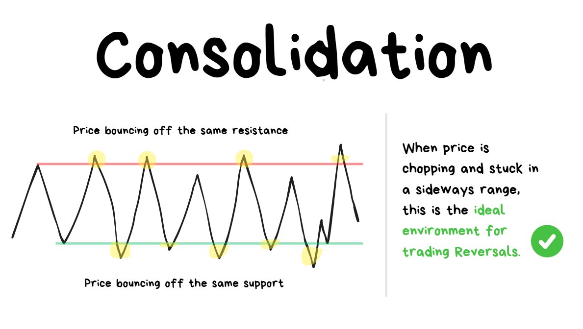
Sideways Price Action = the best for reversals ✅
Consolidation = Chop, price is stuck and bouncing between highs/lows
This is the OPTIMAL environment for trading reversals.
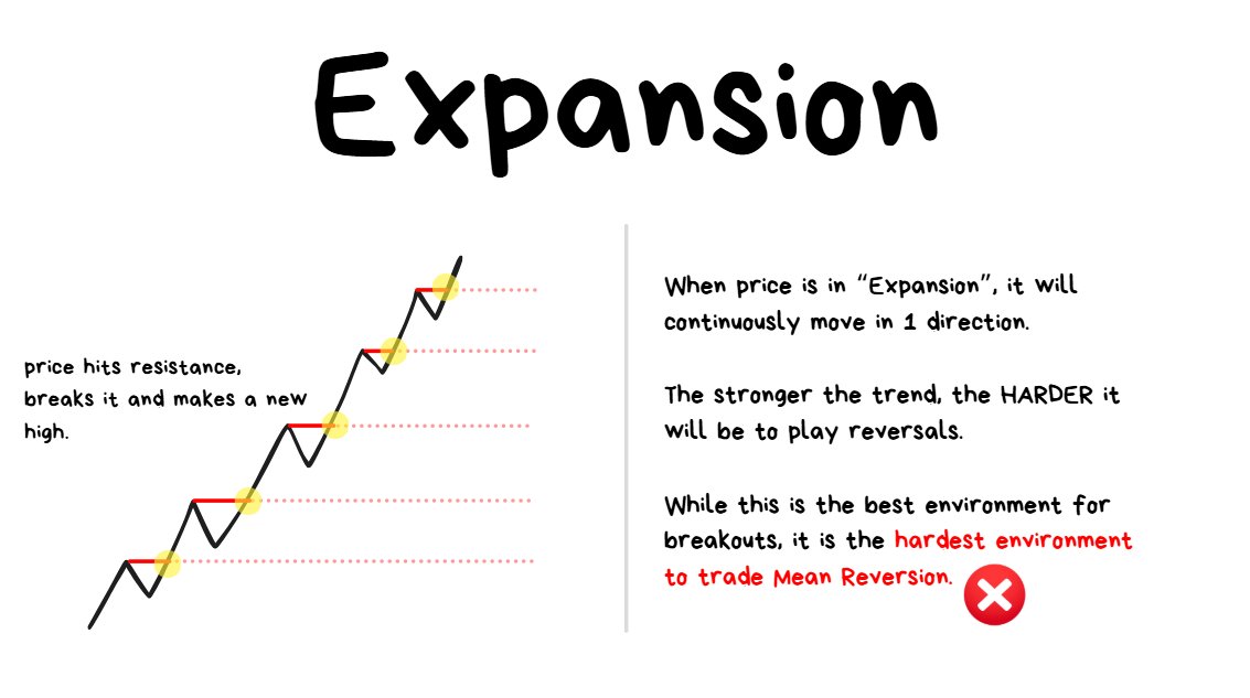
Trending Price Action = the worst for reversals ❌
Expansion = Trend, price is continuously moving in 1 direction.
This is the WORST environment for trading reversals.
I wrote an entire article on trading Breakouts and what to look out for when trading these.
❗️TIP: The best conditions for breakout trading are the worst conditions for reversals. The worst conditions for breakout trading are the best conditions for reversals. The better that 1 strategy style is understood, the better the opposite style is understood too.
Article below ↓
Jul 31, 2025
Lesson 3: How I Do a Market Scan + Setting Alerts
Before even considering the execution rules (entry/stoploss/target) , it is more important to identify the optimal trading environment first.
KITE FLYING ANALOGY ↓
- Imagine you are betting on whether your kite will fly outside or not.
- You can either try really hard to optimize how aerodynamic the kite is OR you can optimize how well you read the weather conditions.
- If there is a hurricane outside, it doesn’t matter how poorly designed the kite is. Even if the aerodynamics are terrible it will still fly.
- If there is literally no wind outside, it doesn’t matter how perfectly designed the kite is… it just won’t fly.
- Therefore it is MUCH more important to be able to read the weather conditions rather than perfectly designing the kite.
the kite = your trading strategy
the weather outside = the current market conditions
There are 2 steps I go through to perform a Market Scan:
- 1 ) Checking Directional Bias on Velo
- 2 ) Flagging “potentially interesting” coins from both Velo + Orion
Will get into the 2 steps below ↓
Step 1: Checking Directional Bias
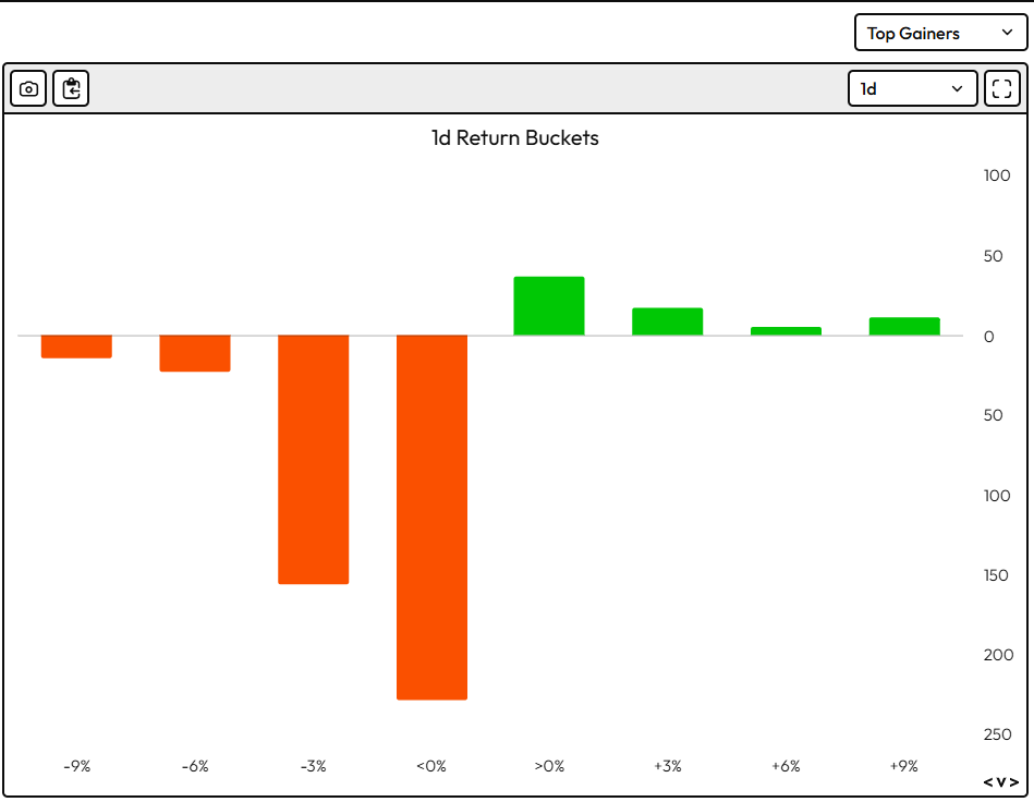
bearish directional bias
Quick shoutout to @velo_xyz for building a fantastic data analytics platform. 🤝
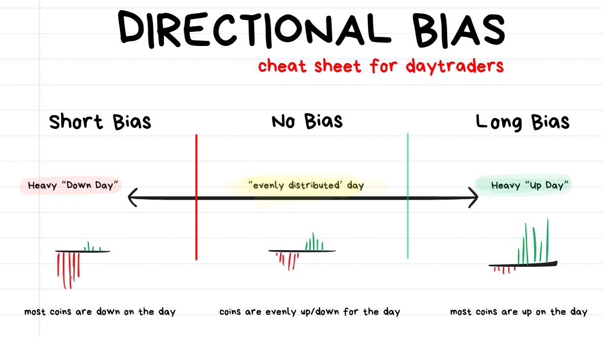
directional bias cheat sheet.
When trying to get a directional bias from Velo (or from whatever screener you prefer to use), there are 3 possible outcomes:
- Most coins are severely down on the day. (Bearish Bias)
- Most coins are evenly distributed with returns. Some coins are up, some are down. (No directional bias)
- Most coins are insanely up on the day (Bullish Bias)
The MAJORITY of the time I will proceed with Option 2, since most coins are evenly distributed with their returns on most days. This is fairly normal and it’s totally fine to NOT have a directional bias on a particular day.
The MINORITY of the time I will proceed with Option 1 and Option 3, since it is an outlier event (rare situation) where every Altcoin is going absolutely psychotic in 1 direction.
Here is how I proceed based on my directional bias:
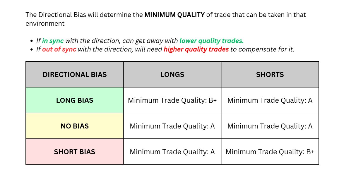
Most of the time I will have “no directional bias” , so to compensate for that I will need to only look for high quality setups.
The only time I can get away with taking lower quality setups is if I have a clear directional bias.
- 🐻Bearish Bias: can get away with lower quality short setups, need to be more strict with higher quality long setups.
- 🐂Bullish Bias: can get away with lower quality long setups, need to be more strict with higher short quality setups.
- ⚠️No Directional Bias: just look for the standard trade setups that I normally do.
Step 2: Flagging Potentially Interesting Coins
Here I will be using both Velo and Orion to help me flag “potentially interesting” coins.
Once I get a list of 5 or 6~ coins, I will then move to Step 3 (which I will talk about further below) and actually do some technical analysis (draw support/resistance levels on the coin and set up alerts) on the coin.
There are 2 main things which make a coin “potentially interesting” for me to trade reversals on:
- 1 ) The coin is mostly going sideways in a range (rather than moving in 1 direction)
- 2 ) The coin has very recently had a big, vertical fast spike (either up or down)
First I’m going to start with the Spaghetti Chart on Velo with top gainers/losers of the day to help me find any potential choppy ranges.
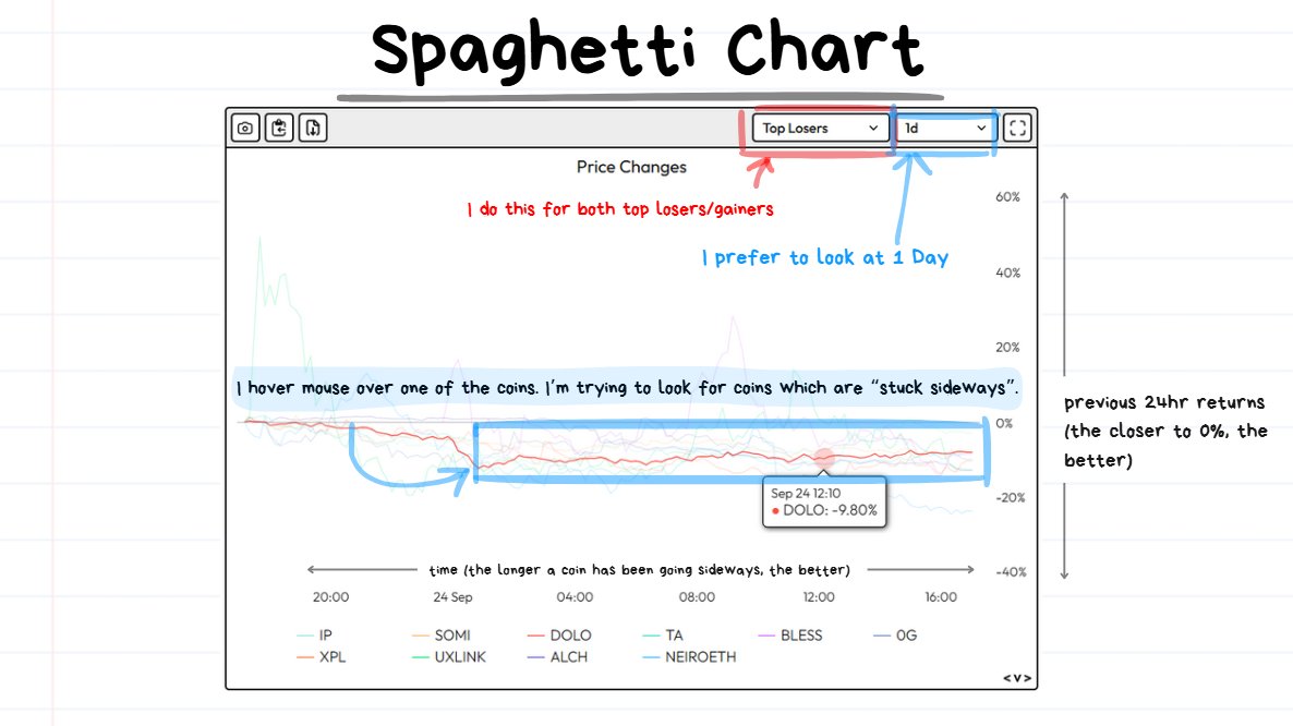
top gainers/losers in prev 24hrs
find coins which are stuck and going sideways for long periods of time.
Any time a coin somewhat interests me I flag it on my TradingView watchlist.
⚠️Note: when flagging, I am preparing a list of coins to do some technical analysis on for the next step.
↓
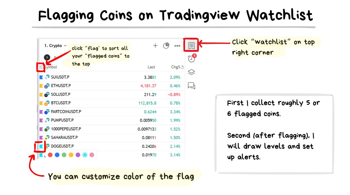
↑ The process of how I flag coins on Tradingview watchlist + “sorting” by flag.
Secondly I move over to Orion Terminal.
Here I will be scrolling down through the list of all Altcoins (except “majors” like BTC, ETH, LTC, XRP .. etc… ).
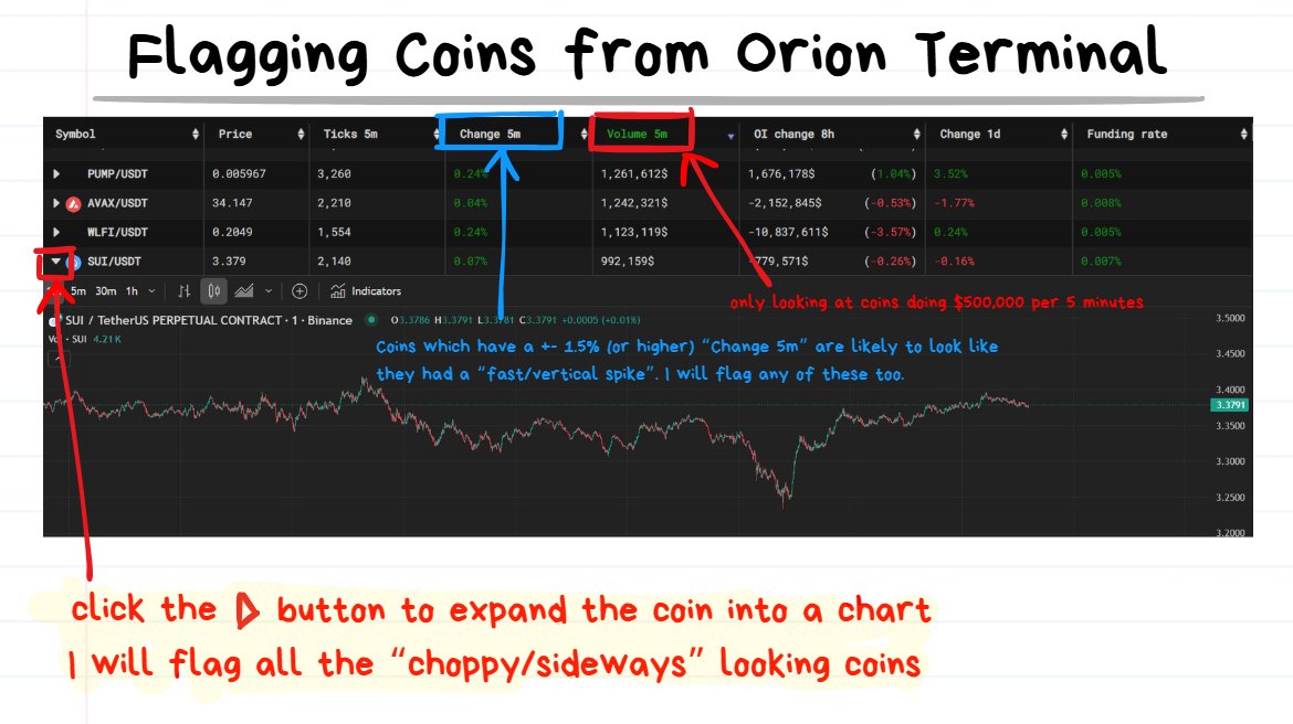
↑ my process for flagging coins from Orion Terminal
I’m mainly looking for the volatile, lower cap Altcoin Perps which are doing at least $500,000 of volume in the previous 5 minutes.
I’ll be looking for the exact same 2 things as I was on Velo:
- 1 ) I’ll be quickly skimming through all charts of coins which are doing at least $500k in the prev 5 minutes and flag any coins which look like a “Choppy/Sideways Range”
- 2 ) I’ll be using the “Change 5M” to help spot any coins which have recently pumped or dumped more than 1.5%. It’s likely that a big 1.5%+ or higher in just 5 minutes of time will show a “fast vertical spike” in the price action which is really nice for trading reversals. I’ll talk more about this further down in this article.
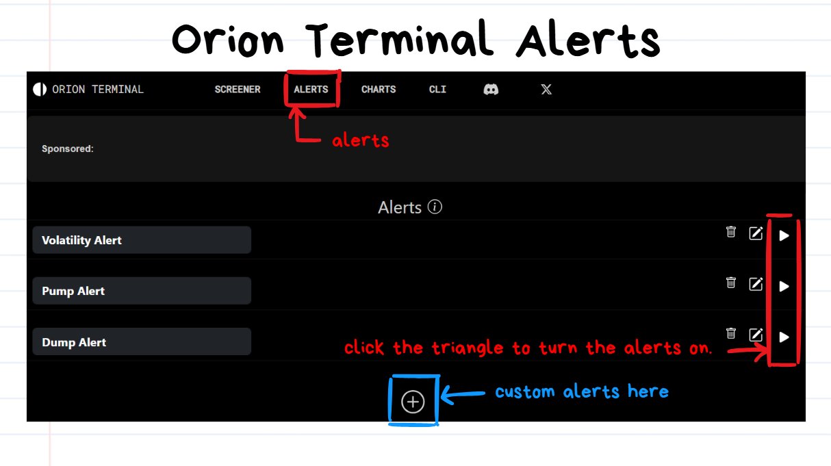
Alerts from Orion Terminal alerts will make it easier to spot fast moving coins.
❗️TIP: Setting up alerts on Orion is fairly straightforward and can be really useful to be notified whenever a coin is moving quite fast.
Lesson 4: Support/Resistance Levels + Setting Alerts
At this point I would have flagged about 5 or 6 “somewhat interesting” coins to trade for the day but I haven’t done any analysis on any of them.
The next 2 immediate steps I have to do are:
- Draw Support/Resistance levels on each of the flagged coins
- Setting up Alerts
In this section of the article I will be talking about “where” I like to trade. I’m going to explain the details of “how” I trade a bit further down.
Picking the levels I trade at ↓
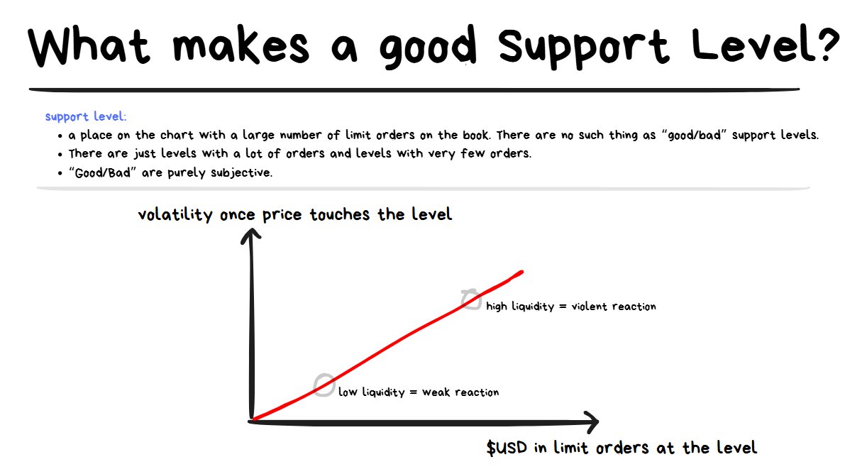
The bigger the level = the bigger the reaction.
The more USD that’s sitting in limit orders at a particular level, the more incentive there is to hit into that limit order with market orders.
The more market orders that are going to come through, the more volatility that I can expect to see shortly after.
I’m mainly looking for swing highs and swing lows ↓

At least 3 candles are required for a swing high/low to be formed.
- Swing Highs = I will be looking for shorts ⤵️
- Swing Lows = I will be looking for longs ⤴️
But I’ll be looking specifically at levels where price has spent “at least roughly” 1 hour away from the swing point.
This is because the more time that price spends away from a level, the more time the market participants have to actually go and place limit orders at a level.
❗️TIP: Generally speaking, the more time that price spends away from a level the more limit orders I can expect to be placed at that level (assuming all other factors are equal).
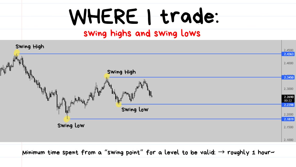
I only bother drawing the 2 fresh swing highs closest to price and the next 2 swing lows closest to price.
There’s no point for me to have 17 different lines cluttering my chart for no reason. I keep it simple.
✏️When Drawing my levels:
- I’ll only look at the next 2 relevant support levels and the next 2 relevant resistance levels.
- This is because it is a waste of my time and attention to have a level drawn at a place where price is nowhere near.
🚨When setting up Alerts:
- I will set 2-3 alerts “on the way” to a level and also another alert directly on the level.
- This is because I want to get notified as price as getting closer to a level so I have time to prepare to make a decision.
- This is much nicer than getting pinged right when price touches the level and then I’m forced to make a split-second decision.
Lesson 5: Entry / Stoploss / Target Rules
Okay so in lesson 4 I talked about “where” I like to trade.
In this lesson I’m going to talk about “how”, so the specific execution of a trade.
There are 2 main ways that I use to trade Reversals:
- 1 ) Failed Breakout Reversals
- 2 ) Fast Spike Reversals
I will give the text explanation + screenshot examples below.
Failed Breakout Reversals
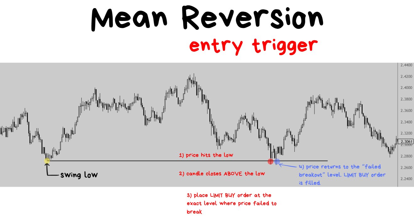
1. price hits a low
2. price rejects the level (1 candle close back above the low. It can be within the same candle or after N candles. Price just needs to close ABOVE the level again.)
3. Limit Buy Order gets placed on the exact same level that just got rejected.
- 1 ) Entry: Price must touch a level, reject it, and then close back on the other side.
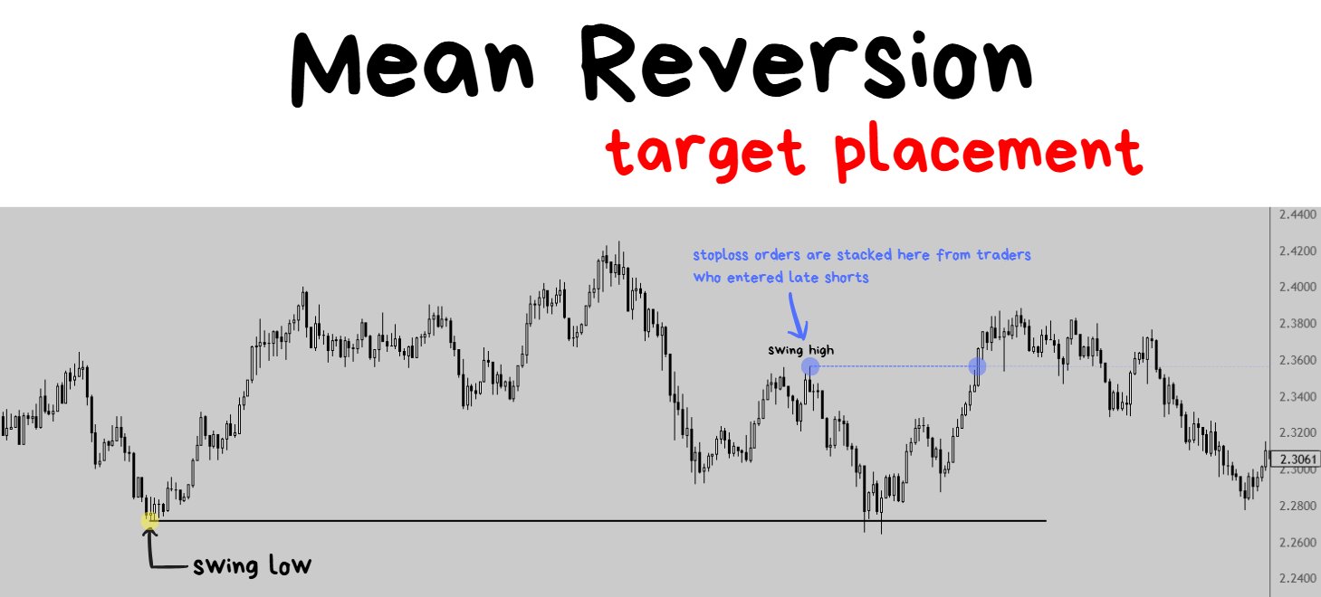
target: some swing point to the upside. Ideally a place where stoploss orders from counterparty are resting.
- 2 ) Target: the next S/R level (swing point). Since my target is going to be a “limit order” , I want to be getting out where market orders will be executed. This means ideally I will be taking profit where breakout traders are being stopped out.
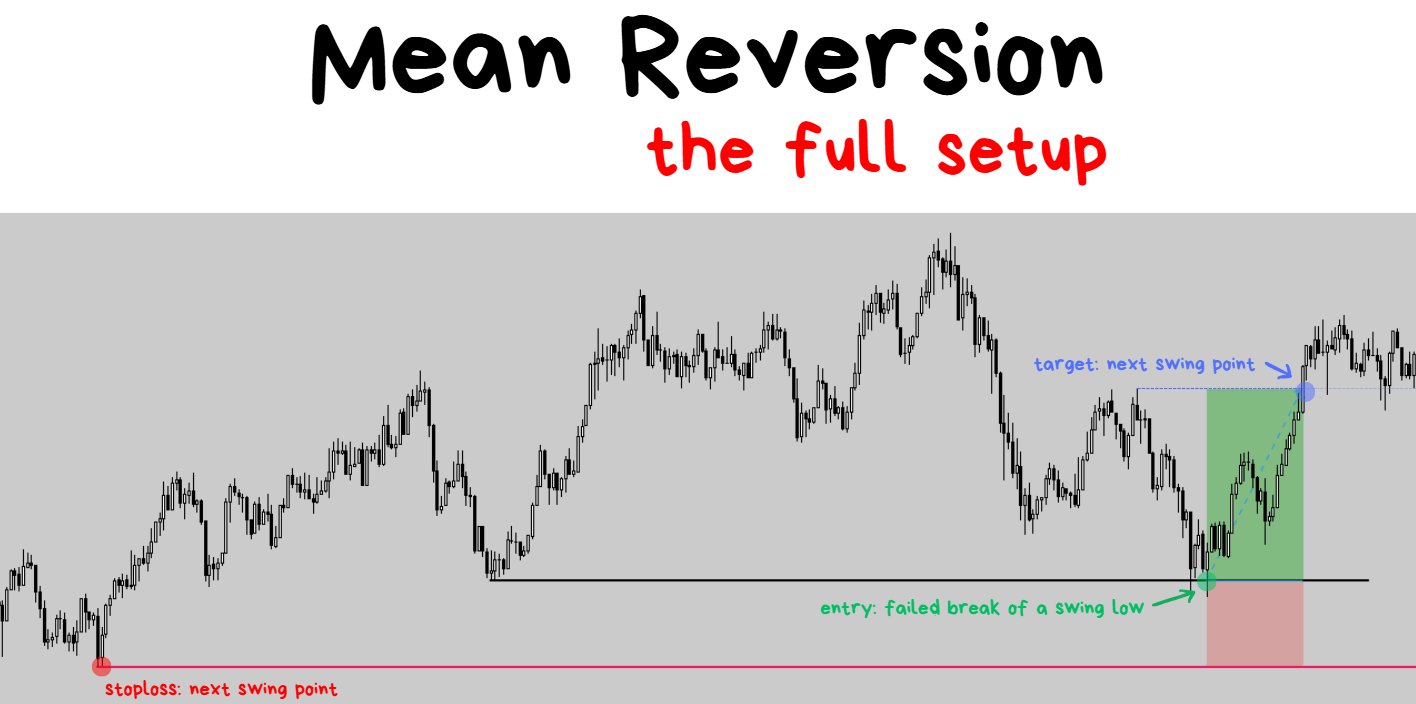
stop is placed at the next available low.
--> I prefer to frontrun these by at least 1 tick to give my stoploss order a higher priority in the trading engine. This will reduce my slippage risk in the event that I do get stopped out.
- 3 ) Stoploss: where the next swing point is (in the same direction). I often go for 1-1.5R trades. In rare cases will go for 1.5R or higher.
Fast Spike Reversals
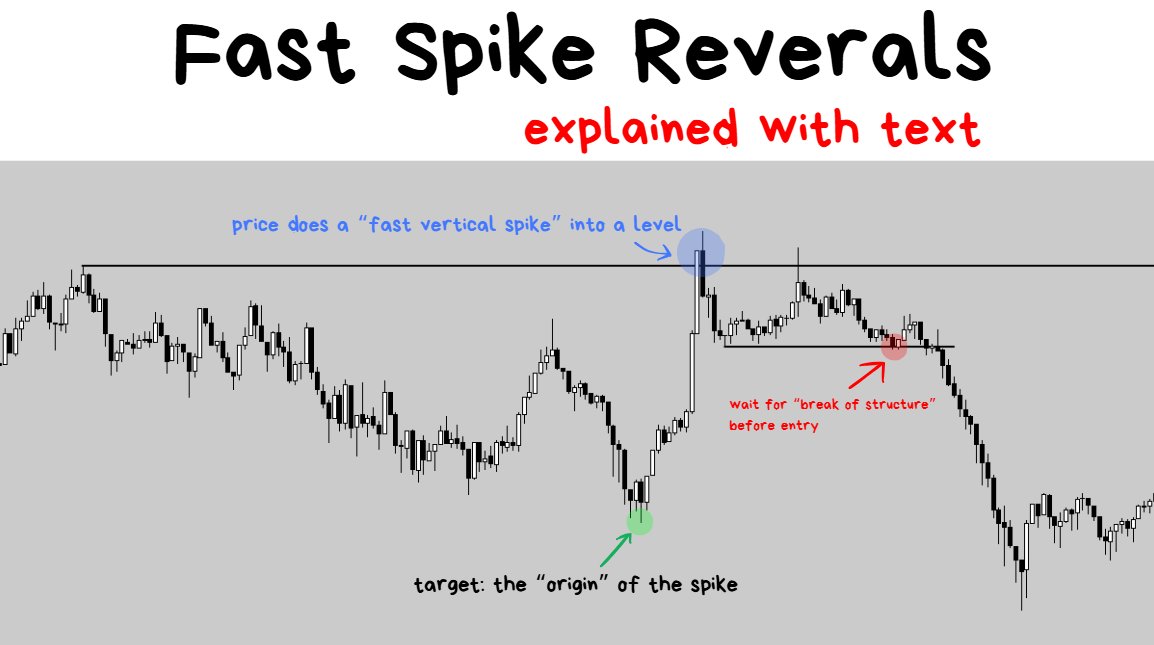
Trade Execution example below ↓
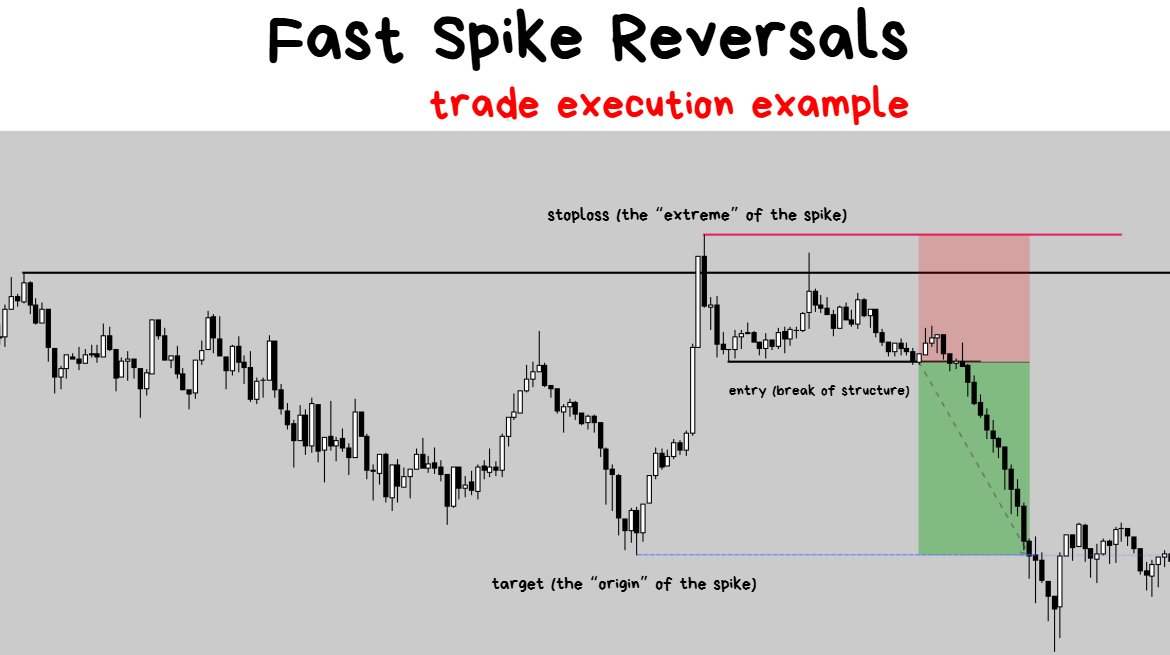
- 1 ) Entry: Price “spikes” into a level, rejects it by closing back underneath the level. My entry will come as soon as a “Break of Structure” happens.
- 2 ) Stoploss: The “highest point” of the spike, after the structural break.
- 3 ) Target: The origin of the spike OR a standard 1R target (1R = equal distance from entry to stoploss).
Lesson 6: How I Determine Trade Quality (Low / Medium / High)
So the important thing to understand when trading ANY strategy is recognizing that not all trades are the same even if they have the same entry/exit rules.
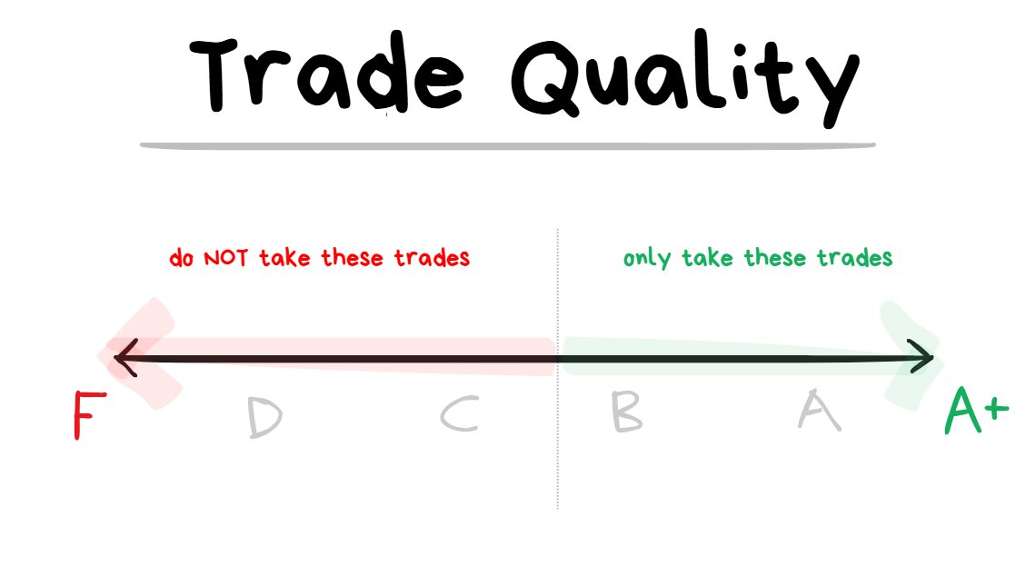
Take LESS bad trades + Take MORE good trades
= make more profit
These are the Top 3 Variables that I use to determine the quality of a trade ↓
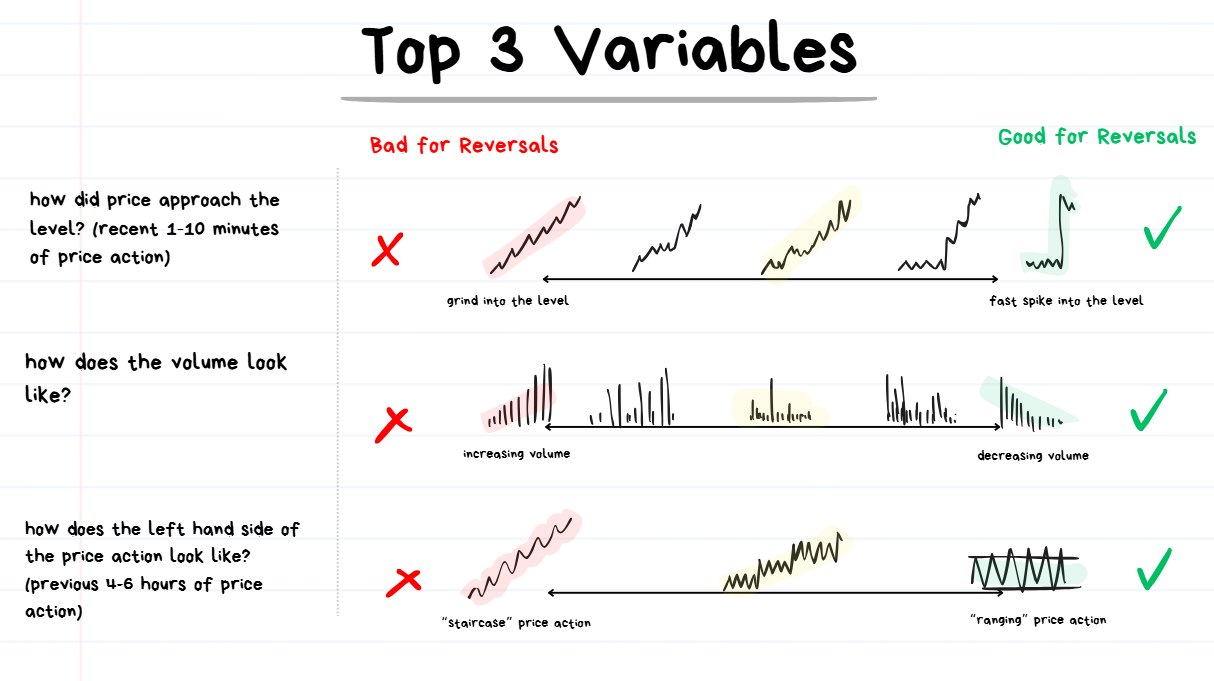
the middle (highlighted in yellow) is when it’s hard to tell if the variable is on 1 extreme or the other.
It’s not good/bad for breakouts or reversals.
- Variable 1 ) How did price approach the level? (ideally a fast spike)
- Variable 2 ) What did the volume look like? (ideally decreasing)
- Variable 3 ) How does the left hand side of the price action look like? (ideally choppy range)
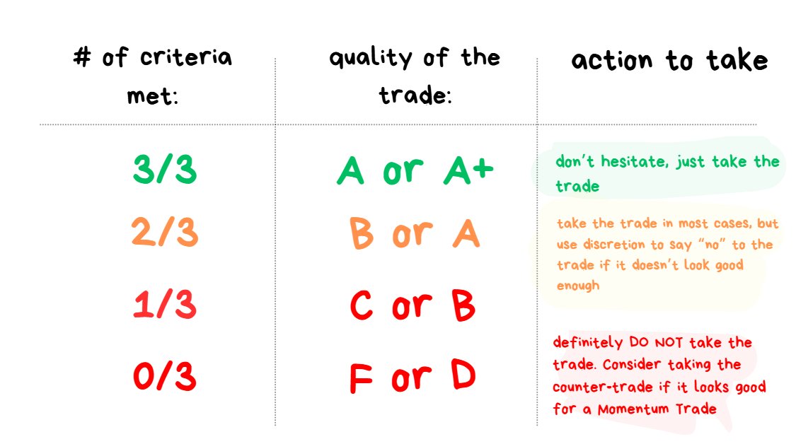
↑ Cheat Sheet : criteria met v.s. trade quality
The more variables that are aligned with each other = the higher the quality of the trade.
The more conflicting variables there are = the lower the quality of the trade.
- ✅3/3 Variables Aligned✅: On the highest quality setups I will be risking the most AND going for wider targets
- ⚠️2/3 Variables Aligned⚠️**:** Most of the time the market won’t provide me with perfect setups. Most of the time they will be imperfect with 1 variable working against me. This is fine and not a problem as long the trade is “mostly” leaning in my favor (This is when 2/3 variable are aligned). Here is where I will need to use my discretion to say “no” and refuse to trade some of the lower quality looking ones.
- ❌1/3 or 0/3 Variable Aligned❌: I absolutely would NOT take the trade. Here is when I actually consider taking the opposite trade (the breakout) since these situations are really poor for reversals.
High Quality Trade Example
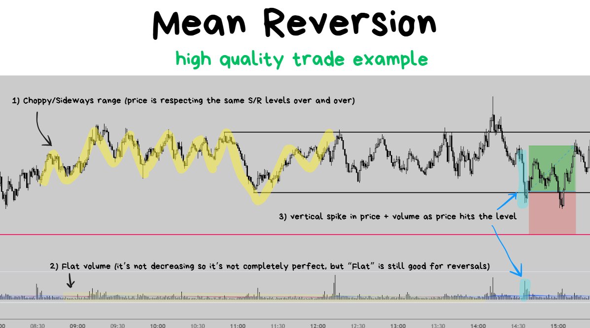
- How did price approach the level? Fast Spike✅
- How did the volume look like? Flat⚠️(it’s not perfect, but it’s still acceptable)
- How did the left hand side of the chart look like? Very Choppy/Sideways✅
Low Quality Trade Example
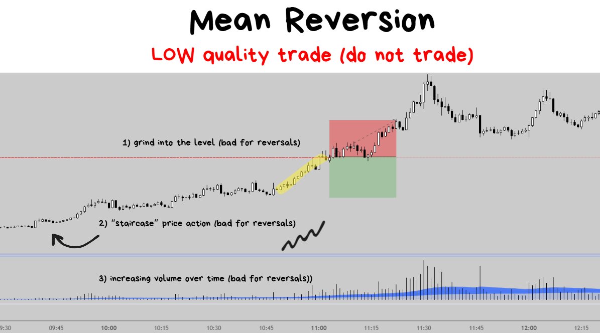
- How did price approach the level? Slow Grind ❌(bad for reversals)
- How did the volume look like? Increasing❌(bad for reversals)
- How did the left hand side of the chart look like? Staircase Price action❌(bad for reversals)
❗️TIP: A coin with price action + volume like this is much better for the Breakout Trade rather than a reversal.
⚠️ Note to Reader
- Unfortunately X Articles has image/media limits
- I am constrained with how much information I can squeeze into this article.
Before moving onto the final Lesson 7, I’m going to do my best to squeeze in all the Extra Tips I think are important to think about when trading reversals below ↓
Extra Tip #1: Time Before the Structural Break
Sep 15, 2025
Observation with trading Fast Spike Reversals on the 1 minute timeframe • The Less Time it takes for the structure to break, the better it is for the reversal trade. • The More Time it takes for the structure to break, the worse it is for the reversal trade.
Extra Tip #2: Volume at the Extreme End of the Spike
Aug 28, 2025
Strategy to make money off Trapped Shorts: • price “spikes” a level while stuck in a range • breakout Shorts enter and get trapped • long after a break of structure • price returns to the origin of the spike • exit for a profit at the origin of the spike Simplified↓
There is only 1 thing that actually moves price, and that’s “executed Market Orders”. ↓
People can OPEN positions with a market order and people can also CLOSE positions with a market order.
But the importance thing to remember here is:
- OPENING a position is VOLUNTARY. You have a choice if you want to open a long position when price starts to reverse.
- CLOSING a position is COMPULSORY. If price starts moving in the opposite direction that you want it to, you will be FORCED to close it for a loss with either your Stoploss or Liquidation being triggered.
❗️TIP: In order for the price to move from your Entry to Target, you will need market orders to be executed AFTER you enter the trade.
I need other traders to OPEN and/or CLOSE a trade after my Entry.
As mentioned above, OPENING IS VOLUNTARY and harder to compete against (because this is a game of speed with other competent traders who are trying to jump into the same trade idea as me).
However since CLOSING IS COMPULSORY, this is a much more reliable metric.
❗️TIP: The more traders that are trapped and then close their position = the more pressure they put on the price to move to my target.
Compare the 2 examples below ↓
- Example 1: $100k of short positions are trapped. By the time half of them close out of their positions only +$50K of market buys have been executed. A mere $50k of market buys isn’t going to move price up by much, even in thin orderbooks.
- Example 2: $5M of short positions are trapped. By the time half of them close out of their positions an entire +$2.5m of market buys have been executed. Price is likely to move upwards a good distance with +$2.5m of market buys in pretty much any altcoin perp.
THE POINT:
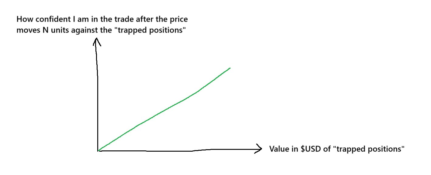
The more USD that is stuck in “trapped positions” , the more confident I get in my trade as the price starts to move against them (and in favor of me).
More trapped positions = more fuel to the fire (i.e. the market can move more once they start to close for a loss)
This is why it’s really crucial for “Step 1” of how I trade these fast spike reversals to be: “price FIRST hits a major level where there was a lot of limit orders”.
Lots of Limit Orders = more Fuel for the fire.
Visualized ↓
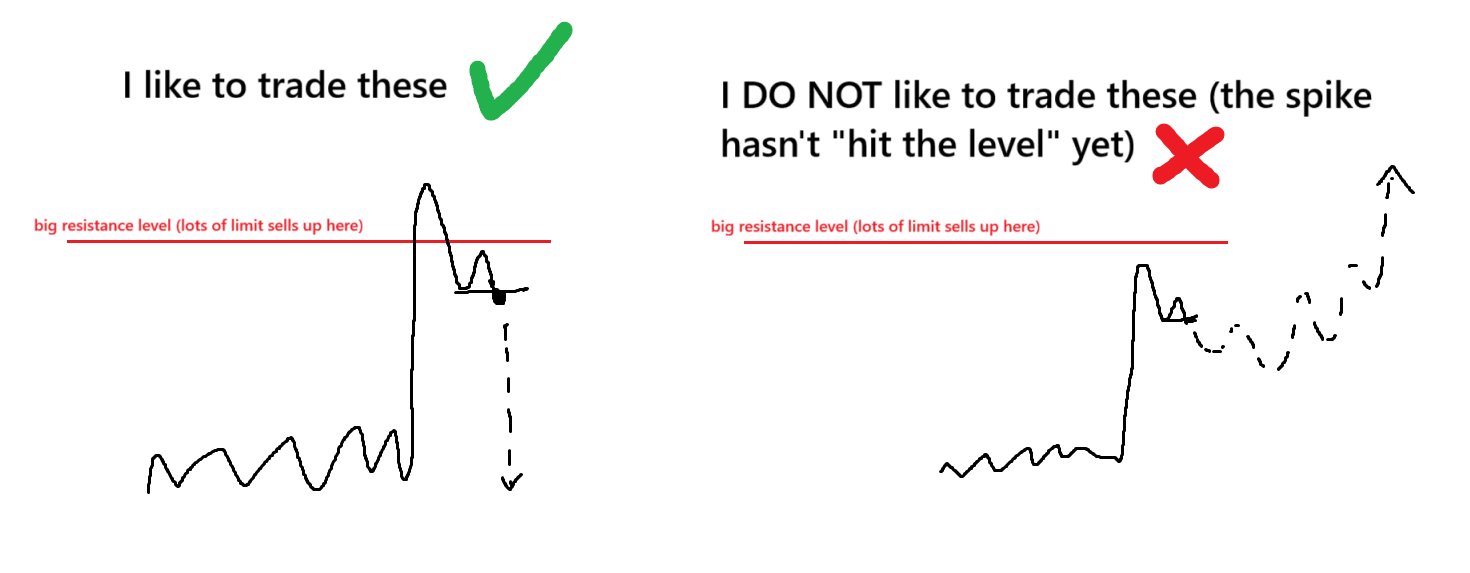
“fast vertical spikes” which serve a key level are harder to trade. Sometimes they will stall a bit and then go for another leg up.
Extra Tip #3: Using MAs or VWAP to Judge the Regime
Nov 4, 2024
Free Alpha: “number of times price tagged MA in previous N candles” if the number is closer to 0 = Trendy Environment if the number is further from 0 = Choppy Environment You’re welcome.
The above can apply to any form of Moving Average, so whether you use MA, EMA, VMA, VWAP or any form of “averaged out price” the concept remains the same.
- No touches of the MA = more likely to be a trending environment. (bad for reversals) ❌
- LOTS of touches of the MA = more likely to be a choppy/sideways environment. (good for reversals) ✅
Lesson 7: How I Cut Losing Trades Before the Stoploss
Before diving into this topic I want to give some quick context first:
My trading profits at the end of the month are going to be based on the total “expected value” (EV) that I am able to extract from the market.
There are 4 variables which will determine how much EV that I can get each month:
- 1 ) Frequency (avg. # of trades taken per month)
- 2 ) Average size of Win
- 3 ) Average size of Loss
- 4 ) Winrate %
This Lesson is about making Variable #3 (Average size of Loss) go down while keeping everything else stay pretty much the same.
If we lose less on our losing trades while keeping everything else the same, then expected monthly profit will go up.
In order to cut a trade early, before the stoploss is hit, I need an “invalidation”.
An invalidation is a condition, such that if it is met, is a sign that my idea “is no longer valid” or “wrong”.
❗️****TIP: I like to use IF → THEN statements. IF X happens, THEN market close the trade.
Price-Based and Time-Based Invalidations
1 ) Price-Based Invalidation:
- IF the “price action does something specific” → THEN market close out of the trade
2 ) Time-Based Invalidation:
- IF “enough time passes” → THEN market close out of the trade.
1. Price-Based Invalidation
There are 2 terms I have to quickly define before getting into this:
- MAE = Maximum Adverse Excursion
- FTA = First Trouble Area
Aug 6, 2025
Every Trader should know this: MAE and MFE ↓
The better I know the average distance that price travels against me on my winning trades, the better I will know how much “breathing room” I need to give to my trades.
Example: let’s imagine that winners, on average, will go -0.3R against me before hitting the target
- If price is currently -0.2R against me, I have no reason to panic. The trade is still behaving like an “average winning trade”. I need to just patiently sit in the trade.
- If price is currently -0.8R against me, I should seriously consider closing out of the trade. This is because this is an abnormal amount to be “offside” in a trade. My winners don’t normally go this far against me, so it makes more sense to just consider closing out of it.
Aug 2, 2025
How I cut trades and take smaller losses: If candle close through the FTA = cut the trade FTA (first trouble area): • a level which is on the way to the stoploss • ideally placed at a level roughly near -0.5R Example ↓
My rule for cutting trades before the Stoploss hits:
- IF “1 candle closes through the FTA” → THEN “market close out of the trade.”
The FTA is a “First Trouble Area” , which is just a level on the way to the stoploss.
The way I place the FTA is going to be dependent on the average MAE of the trade I’m taking:
- Higher Quality Trades = have lower MAE = will require tighter FTA placement (less breathing room)
- Lower Quality Trades = have higher MAE = will require wider FTA placement (more breathing room)
In other words, the higher the quality of the trade, the easier it will be able to tell if my idea gets invalidated early and the easier it will be cut the trade (to take a smaller loss).
❗️TIP: If you collect data on the maximum drawdown of your winning trades you will be able to discover what your average MAE values per winning trade are. Knowing this number will make it easier to cut your losses faster + more accurately.
2. Time-Based Invalidation
🤔QUESTION: 🤔
- My average winning trade takes about 45-60 minutes to play out. If I’m stuck in a trade for 600 minutes, is it behaving like a normal winning trade?
💡ANSWER: 💡
- No, it is not behaving like a normal winning trade.
🧠THE POINT: 🧠
- The more ABNORMAL my active position is when compared to my average winning trades, the more reason I have to CUT the trade early and just get out.
- I want to GET OUT of trades which ARE NOT BEHAVING like my average winners.
- I want to STAY in trades which ARE BEHAVING very similar to my average winners.
Below I wrote a Thread explaining everything with Time-Based Invalidations. ↓
Sep 17, 2025
In this THREAD I will explain “Using Trade Duration to exit Bad Trades faster” I will cover: • Findings from my own trades • How to get these findings on your own • Practical Tip to cut “outlier trades” early to prevent unnecessary losses
Conclusion
If you made it to the very end of this article, well done. 🫡
Here is a quick Summary of the 7 Lessons:
- 1 ) Mean Reversion Trading is betting on price “bouncing” from a level rather than “breaking through” a level.
- 2 ) Mean Reversion is easier to trade in “ranging” environments rather than “trending” environments.
- 3 ) I always do a “Market Scan” before I begin a trading session. My goal is to get a feel for the current market environment as well as pick out some potentially interesting coins.
- 4 ) I’m always going to be trading at swing highs and swing lows. I setup multiple alerts on the way to the level to make sure I get notified as price is approaching the level. I want to have plenty of time before I make a decision.
- 5 ) I trade “failed breakouts” and “fast spike reversals”. They are both based on the same underlying idea. Price hits a level, breakout traders enter, price starts rejecting from the level, the breakout traders are trapped offside, I enter the trade, as the trapped traders start closing their positions the price will move closer towards my target.
- 6 ) There are 3 important variables I consider for all reversal trades. The approach into the level (the recent 1-10minutes). The volume. How the left hand side of the price action looks like (the previous 4-8 hours).
- 7 ) I cut my trade if I get a candle close through the FTA. Where I put my FTA is based on my MAE data.
Once again I appreciate you giving your time and attention to read this article. Don’t hesitate to write any questions you have in the comments. Thank you. 🙏
Source
Written by @spicyofc · View original post · Published: 2025-07-31
Build a Portfolio From Scratch

I am going to break down why most people with high incomes never build real wealth and I’ll share the complete step-by-step framework to fix that starting today.
Let’s get straight to it.
Bookmark This - I’m Roan, a backend developer working on system design, HFT-style execution, and quantitative trading systems. My work focuses on how prediction markets actually behave under load. For any suggestions, thoughtful collaborations, partnerships DMs are open.
You earn well. Maybe very well. But here is the uncomfortable truth. Ronald Read a janitor. He worked low wage jobs his entire life. He drove a used car. He wore a coat held together with safety pins. When he died in 2014, he quietly left behind an $8 million estate, nearly all of it donated to his local hospital and library.
He did not inherit it. He did not get lucky. He built it. Slowly. Systematically. Using a framework so disciplined that it compounded for decades while nobody was watching.
Now think about how many people you know who earn ten times what Ronald Read ever earned and have almost nothing to show for it. The money comes in. The money goes out. The portfolio is a random collection of assets picked on a good day with no real structure underneath.
That gap between earning and building is not about intelligence. It is not about access to special information. It is about knowing the actual framework.
I spent months working inside an equity fund watching something that still bothers me. The sharpest analysts I have ever met were completely right about a market and still lost money on their positions. Right thesis. Right data. Wrong outcome. The reason took me a long time to fully understand. They were not wrong about markets. They were wrong about construction. They had great ingredients and no system around them. In portfolio management, the system is everything.
Warren Buffett said it better than anyone: “Risk comes from not knowing what you are doing.” This article is about knowing exactly what you are doing, step by step, from nothing.
By the end of this article you will understand why most portfolios fail before they are ever truly tested by the market, the mathematical reason why combining assets the right way is more powerful than finding the best single one, the institutional allocation framework that consistently outperformed simple stock and bond portfolios on a risk adjusted basis across full market cycles, the position sizing mathematics that separate people who compound wealth for decades from people who get wiped out right before the market recovers, and the complete monitoring system that keeps everything aligned with its purpose as markets shift around it. If you implement what is in this article, you stop guessing and start building a portfolio with a real mathematical reason to grow.
Note: This article is deliberately long. If you are looking for a shortcut to build brilliance, this article is not for you.
Part 1: The Two Questions That Determine Everything Before You Buy a Single Asset
Most people start building a portfolio by asking the wrong question.
They ask: what should I buy?
The right first question is: what does this money need to do and how much pain can I actually survive on the way there?
These sound similar. They produce completely different portfolios. And the order in which you ask them determines whether you end up with a structure or just an expensive collection of bets.
If you do not define what the money is for, you cannot know when you have won or lost. Building wealth over twenty years needs a completely different structure than protecting capital you need in three years. The assets that are perfect for one goal are dangerous for the other.
The second question is even more important, and most people lie to themselves when they answer it. How much of a loss can you genuinely absorb before you break your own plan?
This is what serious investors call the risk budget. It is the maximum annual loss you can handle without making an emotional decision that destroys the compounding you were building. If a 30% decline would cause you to panic and sell, your real risk budget is less than 30%, no matter how calm you feel right now.
Charlie Munger put it plainly: “It is not supposed to be easy. Anyone who finds it easy is stupid.”
Every proper allocation framework starts with exactly these two inputs. The return your money needs to produce, and the drawdown you can genuinely survive without breaking your behavior. Not what sounds impressive. What is actually true for you.
The math behind this is clean. Your portfolio’s expected return is:
Rp = w₁R₁ + w₂R₂ + … + wₙRₙ
Every asset you hold contributes to your total return in proportion to how much of your portfolio it represents. That is the output you are optimizing. But you cannot optimize an output without knowing what you are solving for and what the hard limits are.
Before you move forward, do this. Write one sentence about what your portfolio needs to accomplish and by when. Then write the largest annual loss you could experience without changing your behavior. Those two numbers are your foundation. Everything in this framework is built on top of them.
Part 2: Why Combining Assets Beats Picking the Best One Every Time
Here is the single insight that separates portfolios that compound from portfolios that just exist.
Combining the right assets together is more powerful than finding the best single asset.
This sounds simple. The mathematics behind it is what makes it extraordinary.
The key variable is correlation. Correlation measures how two assets move relative to each other. It runs from −1 to +1. A correlation of +1 means they move together perfectly. A correlation of 0 means they are completely independent. A correlation of −1 means when one goes up, the other goes down by the same amount.
The portfolio variance formula makes the power of this number precise:
σ²p = wᵀ × Σ × w
Where w is the vector of your asset weights and Σ is the covariance matrix of your holdings. This formula tells you something most people never realize. The total risk of your combined portfolio is not the average of individual risks. It depends entirely on how your assets move together.
Here is an example that makes this impossible to ignore.
Take two assets. Same expected return. Same volatility. In year one, Asset A doubles and Asset B falls 50%. In year two, Asset A falls 50% and Asset B doubles. Held individually, both return zero over two years. You start with 100. You end with 100. Two years of your capital deployed and nothing gained.
Now hold them 50/50 together with annual rebalancing. At the end of year one you sell some of the winner and buy some of the underperformer to restore the 50/50 split. Do the same in year two. The combined portfolio ends with a positive compounded gain. No prediction. No market timing. No special information. Just the mathematical benefit of combining two assets that do not move together and rebalancing systematically.
That is what Harry Markowitz was describing when he earned the Nobel Prize in Economics in 1990 for this exact framework. The free lunch of finance is not about being smart enough to pick the right stock. It is about being disciplined enough to combine the right assets and let the mathematics do the work.
But here is where almost every portfolio quietly fails this test without the investor knowing.
Holding twenty different stocks looks like diversification. But if every one of those twenty stocks responds primarily to the same force, which is the direction of the broad equity market, you do not have twenty independent positions. You have one position expressed twenty different ways. The number of assets is irrelevant. The independence of their return drivers is everything.
The academic concept that captures this precisely is the effective number of independent bets. A portfolio of twenty highly correlated assets may carry the actual risk of only four or five truly independent ones. The investor thinks they are protected. The mathematics says otherwise.
The deeper problem is that correlation is not stable. During calm markets, different asset classes show low or even negative correlation. During a real crisis, when everyone is selling simultaneously to raise cash, correlations spike sharply across almost everything at once. The protection you were relying on disappears at exactly the moment you need it most.
This is market risk. It is the one form of risk that adding more assets cannot solve. You can diversify away company specific risk by holding many companies. You can diversify away sector risk by holding many sectors. But when the entire market falls together, everything falls regardless of how many names you own.
Real diversification means holding assets with structurally different reasons to move. Equities driven by corporate earnings. Government bonds driven by central bank decisions. Commodities driven by physical supply and demand. Real assets that protect against inflation. International holdings with different currency dynamics. These are genuinely different machines. They break for different reasons. They recover on different timelines.
John Templeton, who turned modest investments into one of the greatest fortunes in fund management history, built his wealth on exactly this principle. He bought into markets everyone else was afraid of, in countries everyone else was ignoring, precisely because those positions carried genuinely independent return drivers from everything else he held. The independence was not a side effect of his strategy. It was the strategy.
Part 3: The Allocation Framework That Outperformed a Generation of Professional Guesswork
Once you understand that the power of combining assets comes from their correlation structure, the practical question is simply: how much of each asset do you actually hold?
This is the problem Markowitz solved. His framework takes every possible combination of your available assets, plots each one by its expected return and volatility, and identifies the boundary of combinations you cannot improve upon. That boundary is called the efficient frontier.
Any portfolio sitting below the frontier is one where you could have earned more return for the same risk, or taken less risk for the same return, by choosing a different combination. Only portfolios on the frontier are genuinely efficient.
The single most important ratio for finding your best position on this frontier is the Sharpe ratio:
SR = (Rp − Rf) / σp
Your excess return above the risk free rate, divided by your portfolio’s volatility. It tells you how much return you are earning for every unit of risk you are taking. The portfolio on the efficient frontier with the highest Sharpe ratio is called the tangency portfolio. It is where serious long term capital aims to sit.
Now here is the institutional insight that changes everything about standard allocation advice.
The 60% stocks and 40% bonds portfolio that most advisors still recommend by default does not carry 60% of its risk in equities and 40% in bonds. Because stocks are dramatically more volatile than bonds, the equity portion of a standard 60/40 portfolio carries roughly 90% of the total portfolio risk. The allocation looks balanced in dollar terms and is deeply concentrated in a single risk source.
This observation is exactly what led Edward Qian in 2005 to formalize the concept of risk parity. Instead of allocating by dollar amount, risk parity allocates by risk contribution. The goal is to make each asset class contribute equally to the portfolio’s total volatility rather than having one component dominate it entirely.
The risk contribution of each asset is:
RCᵢ = wᵢ × (Σw)ᵢ / σp
Setting all RCᵢ equal produces a portfolio that is genuinely balanced across its risk sources instead of merely appearing balanced in capital terms. In practice this means holding proportionally more of lower volatility assets like bonds and real assets, and proportionally less of equities.
Ray Dalio built Bridgewater’s All Weather portfolio on exactly this principle. His core insight was disarmingly simple: “I cannot know what the economic environment will be in the future, so I need to own assets that perform well across all environments.” Risk parity is how you build that structure. Not by predicting which environment is coming. By building a portfolio genuinely balanced across all of them.
If you want more absolute return from a risk parity structure, you apply modest leverage to the whole portfolio. Because the portfolio is genuinely diversified, moderate leverage increases expected return without the catastrophic downside that leverage on a concentrated position creates. The Sharpe ratio does not change when you apply leverage uniformly. The absolute return does.
Three steps to implement this. Estimate expected returns, volatilities, and pairwise correlations for your asset classes from historical data across different market regimes, knowing these are estimates and not certainties. Solve for the weights that maximize your Sharpe ratio or equalize risk contribution. Scale the resulting allocation up or down to match the risk budget you defined in Part 1.
Before you move to Part 4, do this. Estimate what percentage of your total portfolio risk currently comes from equities. The number is almost certainly far higher than you expect, and it tells you everything about whether your current allocation matches what you believe it to be.
Part 4: The Position Sizing Mathematics That Decide Who Compounds and Who Gets Wiped Out
Here is what almost no market content will say directly.
Most people who lose money in markets are not wrong about direction. They are wrong about size.
They have the right thesis. They cannot survive the drawdown that occurs before the thesis plays out. So they sell at exactly the wrong moment, take the real loss, and then watch the market do precisely what they predicted, without them.
This is not bad luck. It is a sizing error. And it is the most common way intelligent, well researched investors destroy their own compounding.
The mathematical foundation for getting sizing right is the Kelly Criterion, developed by John Kelly at Bell Labs in 1956. For a position with two possible outcomes:
f* = (p × b − q) / b
Where f* is the fraction of your capital to commit, p is the probability of winning, q is the probability of losing (1 − p), and b is the net payout per unit risked. If your edge gives you a 60% win rate at 1:1 odds, Kelly says to commit exactly 20% of your capital. Not more because you feel confident. Not less because you feel cautious. Exactly 20%, because that is the fraction that maximizes your long run compounded growth rate.
Any position size above Kelly produces less compounded wealth over time than Kelly itself, even when your directional view is correct more often than not. This is counterintuitive but mathematically inevitable. Sizing too large does not just add risk. It actively destroys compounding, silently, over time.
The mathematics of loss recovery explain why. A 10% loss requires an 11% gain to recover. A 25% loss requires a 33% gain. A 50% loss requires a 100% gain. A 75% loss requires a 300% gain. The curve accelerates sharply. Every additional point of drawdown requires exponentially more recovery. Kelly sizing keeps you permanently on the right side of this asymmetry.
The practical complication is that Kelly assumes you know your edge precisely. You never do. Your expected return estimates are backward looking approximations that shift as market regimes change. If you overestimate your edge and bet full Kelly on that overestimate, you are unknowingly betting above your true Kelly fraction and silently destroying compounding without feeling it.
The solution is fractional Kelly, adjusted for how uncertain your edge estimate actually is:
f_empirical = f* × (1 − CV_edge)
Where CV_edge is the coefficient of variation of your edge estimate across many historical scenarios, calculated as the standard deviation of your edge divided by its mean. The more uncertain your edge, the smaller your position. This converts Kelly from a theoretical ideal into a practical operating rule.
Warren Buffett’s two rules of investing are famous. Rule one: never lose money. Rule two: never forget rule one. The Kelly Criterion is the mathematics behind how to actually honor those rules in practice.
Part 5: The Complete System Built Into Eight Steps You Can Start Tomorrow
Everything in the first four parts was foundation. This is the actual build.
A portfolio is not a collection of assets. It is a system with a defined purpose, a deliberate structure, explicit risk controls, and an ongoing monitoring process. The difference between a portfolio that compounds across decades and one that quietly fails is almost never the quality of the assets chosen. It is the presence or absence of the system around those assets.
First: Write down your objective and risk budget formally. The annual return your money needs to produce. The maximum annual loss you can absorb without breaking your own behavior. These are your boundary conditions. Every decision in the system lives inside them.
Second: Choose your asset class universe based on genuine independence of return drivers. Domestic equities. International equities with currency exposure. Government bonds. Commodities. Real assets that protect against inflation. Cash that preserves optionality. Each of these responds to fundamentally different economic forces. That genuine independence is what creates the mathematical edge you are trying to capture.
Third: Estimate your inputs honestly. For each asset class, calculate expected annual return, annual volatility σ, and pairwise correlations with every other asset class. Use historical data across multiple market regimes including severe stress periods. These are estimates, not certainties. The framework is robust to imperfect inputs but the inputs must be as honest as you can make them.
Fourth: Solve for your target allocation. Maximize the Sharpe ratio SR = (Rp − Rf) / σp across your universe, or equalize risk contributions using RCᵢ = wᵢ × (Σw)ᵢ / σp. Either approach is structurally superior to allocating by instinct or by whatever dollar amounts feel comfortable with no mathematical basis underneath them.
Fifth: Scale to your risk budget. If the solved portfolio is less volatile than your budget allows and you want more return, apply modest leverage uniformly. If it carries more volatility than your budget allows, shift weight toward lower volatility assets until σp matches your constraint.
Sixth: Size individual positions within each asset class using f_empirical = f* × (1 − CV_edge). No single position large enough that its maximum realistic loss violates your drawdown constraint. Treat correlated positions as one combined exposure for sizing purposes.
Seventh: Write your rebalancing rules before markets move. Define the drift threshold from target weights that triggers a rebalance. Define the drawdown level at which you reduce overall exposure. Define how frequently you will monitor your factor exposures and correlation structure. Rules written in calm protect you in chaos.
Eighth: Run stress scenarios on the full portfolio before committing. What happens if equities fall 40% and correlations across all assets spike simultaneously? What happens if interest rates surge sharply and both stocks and bonds decline together as they did in 2022? What happens if your largest single position loses 60%? Knowing the answers before these events happen lets you design a portfolio that survives them. Not knowing means responding to damage you could have anticipated.
The ongoing maintenance after setup is far simpler than the construction. Every quarter, check whether your actual allocation has drifted materially from the target due to price movements. Check whether volatility and correlation structures have shifted enough to change the optimal target. Check whether any position has grown large enough through appreciation to violate your sizing rules. When triggers are hit, rebalance. That is the entire maintenance process.
Ronald Read, who left behind $8 million on a lifetime of modest wages, was not running a sophisticated quantitative system. But the principle he embodied is exactly the same one underneath every step above. Clear purpose. Disciplined structure. Patience to let compounding work without breaking the plan. He was not smarter than the people who earned ten times what he earned. He was better structured.
You have the earnings. You now have the framework. The only variable left is whether you build it.
The Summary
A portfolio is a construction problem, not a selection problem.
Define what the money needs to do and how much loss you can genuinely absorb. Combine asset classes with independent return drivers so the correlation structure works in your favor. Calculate your allocation using the efficient frontier and risk parity logic so the structure is genuinely balanced rather than just appearing balanced. Size every position using fractional Kelly adjusted for real estimation uncertainty. Set rebalancing and drawdown rules before you need them. Stress test the full structure before you commit to it.
This is how ordinary discipline built an $8 million estate on modest wages. This is how Ray Dalio built All Weather. This is how Markowitz earned the Nobel Prize. The framework has been sitting in plain sight for over seventy years.
Now you have it. Build something with it.
Source
Written by @RohOnChain · View original post
The Quant Roadmap

I am going to break down the exact blueprint to build a $650,000/yr quant career from zero & land roles at firms like Jane Street & Citadel. Let’s get straight to it.
Bookmark This - I’m Roan, a backend developer working on system design, HFT-style execution, and quantitative trading systems. My work focuses on how prediction markets actually behave under load. For any suggestions, thoughtful collaborations, partnerships DMs are open.
The quant industry is not waiting for anyone. Entry level quantitative researchers at Citadel already pull between $336,000 and $642,000 in total compensation right out of college. Jane Street paid its average employee $1.4 million in the first half of 2025 alone. Interns at IMC Trading earn the annualized equivalent of over $240,000. The five year benchmark for those who survive at top prop shops sits between $800,000 and $1,200,000 per year.
And that is before you look at what is happening in prediction markets. The space is expanding fast into elections, economics, sports and geopolitical events. Institutional quants are now deploying systematic strategies in prediction markets the same way they deploy them in equities and derivatives. The same probability frameworks, the same signal combination techniques, the same risk management principles. I already wrote a specific article on getting into Prediction Market Quant.
Feb 24
When I was 16, I had zero understanding of how probability and mathematics actually worked in real markets. Today I lead systematic trading strategies in prediction markets at an institutional level. This happened because I followed a structured path from complete beginner to understanding the mathematical frameworks, technical execution and market microstructure that institutions use to extract edge systematically. AI and machine learning hiring in quantitative finance accelerated sharply through 2025. Every major fund is building systematic strategies powered by ML models. Quantitative analyst demand is projected to grow 9 percent through 2028 and recruiters describe 2026 as possibly the most competitive quant talent market globally.
And yet most people who want to break into this space have no idea how to actually do it.
They think quant trading is about being smart about markets. Picking the right stocks. Having strong opinions on price direction. They picture Wall Street suits and Bloomberg terminals and assume the field belongs to people who studied finance at elite universities. They assume you need MIT or Stanford on your resume. They assume that without an Ivy League name, the door is already closed.
This is completely wrong. And it is the single biggest reason most people never even try.
Jane Street explicitly states on their job listings that prior knowledge of finance or economics is not expected or required. Over two thirds of their recent intern class studied computer science or mathematics. Not finance. Not economics.
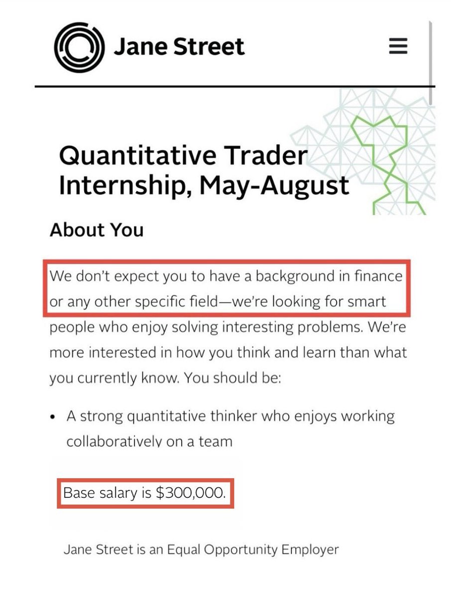
Jane Street Hiring
By the end of this article you will understand what quant trading actually is and why it pays what it does, the four main quant roles and which one fits your background, the complete mathematical roadmap from zero built in the correct learning order, what the interview process at top firms actually tests and how to prepare for it precisely, and the exact staircase from no experience to your first real institutional credential.
Note: This article is deliberately long. Every part builds on the one before it. If you are serious about building a quant career, read every single word. If you are looking for a shortcut, this is not for you.
Part 1: What Quant Trading Actually Is and the Roles Inside It
Most people think quantitative trading is about having opinions on where markets are going.
It is not. Quant trading is about math.
You are working with statistical relationships, pricing inefficiencies, and structural edges that exist because markets are complex systems run by humans who make systematic and repeatable errors. The goal is not to be right about any specific outcome. The goal is to find situations where the mathematical probability is in your favor, size the position correctly and repeat that process thousands of times until the expected value accumulates into real returns.
Think of it the same way a casino operates. The casino does not try to predict whether any single bet will win. It runs the game repeatedly with a small mathematical edge on every bet and lets the law of large numbers do the rest. Quant trading firms operate the same way. They find edges. They size positions correctly. They execute at scale.
This framework applies identically to prediction markets. A systematic quant does not try to predict whether a specific political candidate will win an election. They try to find markets where the implied probability deviates measurably from what the underlying data actually supports, bet on that deviation and repeat across hundreds of events simultaneously. The tools are the same. The mathematics is the same. The edge comes from the same source.
Now the roles, because the preparation required differs significantly across them.
Quantitative Researcher is the highest paid and most demanding role. These are the people who find patterns in massive datasets, build predictive models, and design the actual trading strategies. They need PhD level mathematical and statistical depth, or genuinely exceptional undergraduate achievement in a hard quantitative field. Entry level total compensation at top firms ranges from $350,000 to $650,000 and scales dramatically from there.
Quantitative Trader takes models built by researchers and executes real trades in real time. Fast probabilistic thinking, strong mental math, and confident decision making under pressure with incomplete information. This role has the highest compensation variance of any quant career. Exceptional traders reach eight figures in a single year. Entry level compensation at top firms typically starts between $200,000 and $400,000 with unlimited upside.
Quantitative Developer builds the infrastructure that makes research actually trade in live markets. Trading platforms, execution engines, real time data pipelines, low latency systems. Production level C++, Rust, and Python at very high performance standards. Entry level total compensation typically sits between $200,000 and $350,000 at top firms.
Risk Quant focuses on model validation, value at risk calculation, stress testing, and regulatory compliance. The most stable quant career path with the most predictable compensation trajectory. Lower ceiling than the other three roles but significantly more stability.
The fastest growing role right now is the AI and machine learning focused quant who builds signal generation systems using deep learning, processes alternative data at scale, and deploys ML models directly into live trading environments. This sits at the intersection of quant research and machine learning engineering and it is where the most aggressive hiring is happening across 2025 and 2026.
The misconception to eliminate before reading further: you do not need a finance degree to do any of these jobs. You need mathematical ability, programming skill and the discipline to build the foundation in the correct order.
Part 2: The Mathematical Foundation in the Correct Order
The path from zero to quant-ready is like levels in a video game. You cannot skip levels. Every concept builds on the one before it. If you try to jump to machine learning or options pricing without the foundational layers underneath, you will build surface familiarity with many topics and genuine understanding of none of them. That will not survive a quant interview.
The correct order is five layers deep. Each layer is the prerequisite for everything that follows it.
Layer One: Probability
Everything in quantitative finance reduces to one question. What are the odds, and are the odds in my favor?
If you do not understand probability at a deep level, nothing else in this article matters. Options pricing is a probability problem. Signal modeling is a probability problem. Market making is a probability problem. Position sizing is a probability problem. Prediction market trading is a probability problem at its core.
The most important concept at this layer is conditional thinking. Quants do not think in absolutes. They think in conditionals. Given what I know right now, how likely is this outcome?
The formula that makes this precise:
P(A|B) = P(A and B) / P(B)
The probability of A given B equals the probability of both events happening divided by the probability of B alone.
Here is how this works in practice. Imagine you are building a signal for a prediction market on an economic announcement. The unconditional probability that the market moves sharply after the announcement is 40 percent based on historical base rates. But on days when options implied volatility is significantly elevated before the announcement, the conditional probability of a sharp move rises to 68 percent. That 68 percent is real usable signal. The unconditional 40 percent mixes signal and noise in a way you cannot separate without conditioning.
Bayes Theorem is the other essential concept here. It tells you how to update your conviction as new information arrives:
Posterior = (Likelihood x Prior) / Evidence
Your updated belief equals how likely you would see this new evidence if your hypothesis were true, multiplied by how strongly you already believed the hypothesis, divided by how likely you would see this evidence under any hypothesis. The traders who update their beliefs fastest and most accurately when new information arrives consistently outperform everyone else.
Expected value and variance are the two numbers you will think about for the rest of your quant career. Expected value is your average outcome across all scenarios. Variance is how much your actual outcome can deviate from that average. If your strategy has positive expected value and you can survive the variance long enough for it to accumulate, you will make money. If you size positions too large relative to variance, you will go broke before the expected value has time to work.
Resource for this layer: Blitzstein and Hwang, Introduction to Probability. Full PDF available free from Harvard. Work every problem in Chapters 1 through 6. Budget three to four weeks at two focused hours per day.
Layer Two: Statistics
Once you understand probability, you need to learn to listen to data. That is statistics. The most important thing statistics teaches is that most of what looks like real signal is actually noise.
You build a strategy. It backtests at 15 percent annual return. Is that real edge or lucky variation?
Hypothesis testing is how you find out. Assume the null hypothesis that your strategy has zero true expected return. Calculate how likely you are to see results this strong if that assumption were true. If you test one thousand random strategies, fifty of them will show apparently strong results purely by chance at the standard 5 percent significance level. This is the multiple comparisons problem. It is the single most common reason backtests look great and live trading results are terrible.
Linear regression is the workhorse. Regress your strategy returns against known risk factors and look for the intercept called alpha. If alpha is zero after accounting for all standard factors, your supposed edge is just disguised exposure to things that were already well understood. The only number that matters is the alpha that survives after every known factor is accounted for.
Resource for this layer: Wasserman, All of Statistics, Chapters 1 through 13. Budget four to five weeks.
Layer Three: Linear Algebra
Linear algebra is the machinery that runs everything in quantitative finance and ML. Portfolio construction, principal component analysis, neural networks, covariance estimation, and factor models all run on matrix mathematics.
A covariance matrix captures how every asset moves relative to every other. Portfolio variance collapses to:
Variance = w^T x Sigma x w
Where w is your weight vector and Sigma is the covariance matrix. This single expression is the mathematical core of portfolio optimization and risk management.
Eigenvalues reveal what actually matters inside that covariance matrix. In a universe of 500 stocks, the first five eigenvectors typically explain 70 percent of all variance. Everything else is noise. Eigendecomposition is the foundation of factor investing, dimensionality reduction, and the statistical architecture of large scale systematic strategies.
Resource for this layer: Gilbert Strang’s MIT 18.06 lectures, completely free at MIT OpenCourseWare. Watch all of them. Then work through Strang’s Introduction to Linear Algebra textbook. Budget four to six weeks.
Layer Four: Calculus and Optimization
Nearly every problem in quantitative finance reduces to maximizing something subject to constraints. Portfolio construction, model training, and execution strategy are all optimization problems.
Convex optimization is essential here. A convex optimization problem has a unique global solution that can be found efficiently. Most portfolio construction and risk management problems can be structured as convex programs. Understanding when a problem is convex and how to solve it efficiently is a core practical skill in the field.
Resource for this layer: Boyd and Vandenberghe, Convex Optimization. Full PDF free from Stanford. Work Chapters 1 through 5. Budget four to five weeks.
Layer Five: Stochastic Calculus
Before stochastic calculus you can analyze data and build statistical models. After it you can derive how financial instruments are priced from mathematical first principles. This is the layer where Black-Scholes comes from and where the most sophisticated systematic strategies are designed.
The central insight of stochastic calculus is that in a world with randomness, the square of a small random increment is not negligible the way it is in ordinary calculus. This one fact changes every calculation and produces Ito’s Lemma, the chain rule of stochastic calculus. Apply it to an option price and you derive the Black-Scholes equation:
dV/dt + (1/2) sigma squared S squared (d2V/dS2)+rS (dV/dS) - rV = 0
What makes this result remarkable is that the expected return of the stock disappears completely. The option price does not depend on where you think the stock is going. Only on how much it moves. This was the conceptually radical result that made modern derivatives pricing possible.
Resource for this layer: Shreve, Stochastic Calculus for Finance, Volumes 1 and 2. The gold standard. Budget six to eight weeks and do not rush it.
Part 3: Programming, HFT Tools and the Tech Stack That Actually Matters
There are two completely separate types of programming skill that matter in quant finance and most candidates confuse them.
The first is research programming. Writing clean Python to analyze data, build and backtest statistical models and implement machine learning pipelines. This is what quant researchers and most quant analysts use every day.
The second is production systems programming. Writing high performance C++ or Rust that executes at microsecond latency, processes real time market data, manages order books, and handles execution logic without a single missed tick. This is what quantitative developers and high frequency trading engineers build.
If you are targeting quant researcher or quant analyst roles, Python is your primary tool. Master pandas and polars for data manipulation, where polars runs ten to fifty times faster on large datasets. Use numpy and scipy for numerical computation. Use xgboost, lightgbm and catboost for machine learning on tabular data. Use pytorch for deep learning. Use cvxpy for optimization problems. Use statsmodels for statistical testing.
If you are targeting quantitative developer or HFT engineering roles, C++ and Rust are non-negotiable.
C++ has been the dominant language in high frequency trading for decades. The reasons are control over memory layout, deterministic performance without garbage collection pauses and the ability to optimize code to within nanoseconds of theoretical hardware limits. At firms trading at microsecond or sub-microsecond speeds, a poorly optimized memory access pattern can cost more in slippage than a strategy earns in edge. The relevant C++ libraries are QuantLib for derivatives and financial mathematics, Eigen for high performance linear algebra, and Boost for general purpose utilities.
Rust is the serious emerging competitor to C++ in this space and it is gaining adoption rapidly. Rust provides the same level of performance as C++ with memory safety guarantees enforced at compile time, eliminating entire classes of bugs that regularly appear in C++ codebases. NautilusTrader, one of the most advanced open source trading platforms available, uses a Rust core for performance critical components with a Python API for research and strategy development. This Rust plus Python architecture is becoming the standard pattern for new systematic trading infrastructure. RustQuant is available specifically for options pricing and quantitative derivatives work in Rust.
For data sources: yfinance is free and sufficient for learning. Polygondotio at around $200 per month provides sub-20 millisecond latency and is the standard for serious retail systematic work. Bloomberg Terminal at around $32,000 per year is the institutional standard. Finnhub offers a free tier for early projects.
For backtesting: NautilusTrader for production-grade work. Backtrader and vectorbt are simpler starting points for learning the concepts.
Homework and the interview question that reveals everything:
Here is one of the most famous probability problems that top quant firms use in early screening rounds. It is simple to state, surprisingly deep to solve correctly and directly tests the conditional thinking from Part 2.
You flip a fair coin repeatedly until you get two heads in a row. What is the expected number of flips?
Work through this yourself before reading anything else. Do not search for the answer. The process of setting up the states, writing the equations for each state and solving the system is exactly the type of reasoning quant interviewers are watching for.
Drop your answer and your approach in the comments. There is a specific result this problem converges to and the method you use to get there reveals more about your mathematical thinking than the answer itself.
Part 4: The Interview Process Decoded
Most candidates prepare for what they imagine quant interviews look like. The reality is more structured and more demanding than most people expect.
At a firm like Citadel the interview process spans multiple tracks running simultaneously. Quantitative software engineering, trading and quant research tracks each have different structures and test different things. A serious candidate in a single recruiting season may go through fifteen to twenty separate interviews across all three.
The final rounds are called super days. Six consecutive forty-five minute interviews in a single day. Topics span from low level C++ and system design to probability proofs to machine learning design questions to behavioral interviews with team leads. You need to code cleanly, derive mathematical results clearly, and explain your reasoning out loud at every step.
Mental math speed matters significantly more than most candidates expect. Firms use tools like Zetamac for early screening. Target 50 or more correct answers per minute before applying.
Jane Street designs its interview problems to be intentionally harder than one person should be able to solve alone. They are testing how you use hints. How you reason forward under uncertainty. How you collaborate under pressure. A candidate who narrates their thinking, considers edge cases, and acknowledges uncertainty while continuing to reason will consistently outperform a candidate who goes silent and then produces a correct answer without explanation.
The Green Book, formally titled A Practical Guide to Quantitative Finance Interviews by Xinfeng Zhou, is the single most referenced preparation resource across every candidate who has landed an offer at a top quant firm. Over 200 real interview problems covering probability, statistics, brain teasers, mental math, and finance puzzles. Work through it slowly. Spend at least fifteen minutes genuinely attempting each problem before looking at any hint.
Supplement with QuantGuidedotio for quant-specific practice problems and Brainstellar for probability puzzles at interview difficulty.
For coding rounds, work through the LeetCode Blind 75 problem set with focus on understanding the underlying pattern of each problem type rather than memorizing solutions. Dynamic programming is the most common failure point at final rounds at Citadel and Jane Street specifically.
Research experience is what separates the strongest quant research candidates from everyone else. Not coursework grades. Actual research where you formulated a hypothesis, built something to test it, and can describe precisely what you learned from the process including what failed and why.
Behavioral preparation is consistently underestimated. Practice answering behavioral questions out loud with someone who gives genuine feedback until your answers sound natural. Every final round has a meaningful human evaluation layer that determines outcomes as much as the technical rounds.
Competitions that directly fast-track to employment: Jane Street Kaggle competition with a $100,000 prize. WorldQuant BRAIN which pays cash for alpha signals you submit. Citadel Datathon which explicitly fast-tracks winners into employment interviews.
Part 5: The Staircase From Zero to $650,000 a Year
The single biggest mistake is attempting a vertical jump. Applying directly to Citadel or Jane Street with no credentials, getting rejected and concluding the field is closed.
The field is not closed. They attempted an eighteen stair jump when the process requires one step at a time.
First: Build the mathematical foundation in the correct order from Part 2. Run the academic study track and the practical coding track simultaneously. Do not wait for mathematics to be perfect before starting to code. Both develop in parallel.
Second: Build at least one real project before applying anywhere. Backtest a systematic trading strategy using real historical data and document every assumption and decision you tested. Submit a model to WorldQuant BRAIN or Kaggle and write up what you built. Implement a simple algorithm using a broker API like Alpaca. These projects prove you can translate mathematical knowledge into something functional.
Third: Get your first institutional credential. Cold email PhD students in research labs and ask specifically to contribute to ongoing work. TA a quantitative course. Join a research assistant position. The specific title matters far less than having a real line of technical experience to talk about.
Fourth: Use each credential to reach the next level. Research lab opens startup interview doors. Startup credential opens mid-tier firm doors. Mid-tier firm opens the elite fund doors. Nobody has found a reliable shortcut around this staircase.
Fifth: Apply before you feel ready and track everything. Every rejection is data. Every interview is practice. Build a spreadsheet. Track every application, every online assessment, every interview, and every question you were asked that you could not answer cleanly. Go study that specific thing before the next interview.
Sixth: Compete publicly. The competitions in Part 4 are recruitment pipelines, not just skill building exercises. Firms watch the leaderboards and strong performance has directly led to job offers for candidates who had no prior connection to those firms.
The mathematical foundation is the actual moat. The ability to derive why Ito’s Lemma has an extra term that ordinary calculus does not. To know when a convex optimization approach will and will not work in a live market. That depth separates quants who build real edge from quants who borrow it. Borrowed approaches expire when everyone else adopts them. Mathematical fluency generates new approaches indefinitely.
Before you close this article, write down three specific things. Where you are right now on the staircase. What the next concrete step above your current position looks like. And the single most specific action you can take in the next seven days toward that next step. Not a vague intention. A specific action with a specific deadline.
The Complete Reading List
Mathematics: Blitzstein and Hwang, Introduction to Probability, free PDF from Harvard. Strang, Introduction to Linear Algebra plus MIT 18.06 lectures free at OpenCourseWare. Wasserman, All of Statistics. Boyd and Vandenberghe, Convex Optimization, free PDF from Stanford. Shreve, Stochastic Calculus for Finance, Volumes 1 and 2.
Quantitative Finance: Hull, Options Futures and Other Derivatives. Natenberg, Option Volatility and Pricing. Lopez de Prado, Advances in Financial Machine Learning. Ernest Chan, Quantitative Trading. Zuckerman, The Man Who Solved the Market.
Interview Preparation: Zhou, A Practical Guide to Quantitative Finance Interviews. Crack, Heard on the Street. Joshi, Quant Job Interview Questions and Answers.
The Summary
Entry level quant researchers at Citadel earn between $336,000 and $642,000 in total compensation. Jane Street pays its average employee $1.4 million per year. The five year benchmark at top prop shops sits between $800,000 and $1,200,000 annually. Prediction markets are adding an entirely new systematic trading frontier on top of everything that already exists in traditional quant finance.
The complete path from zero to that level of compensation is documented in this article. Five mathematical layers in the correct sequence. A specific set of resources that actually work. A clear picture of what interviews actually test. A staircase of credentials that each make the next one reachable.
You do not need an Ivy League name. You do not need a finance background. You need the right foundation built in the right order and the discipline to follow the staircase without trying to skip levels.
The information asymmetry that keeps most people out of this field is not about intelligence. It is about not knowing what the path looks like.
Now you know.
Here is the question I want you to sit with.
If the complete blueprint to one of the most financially rewarding careers that exists is publicly available, requires no prestigious background, and can be followed starting from wherever you are right now, what is actually stopping most people from beginning today?
Drop your answer in the comments. And while you are there, drop your answer to the coin flip problem from Part 3 as well.
There is no wrong answer but there are very revealing ones.
Source
Written by @RohOnChain · View original post · Published: 2026-02-24
Markov Chains — Regime Detection Framework
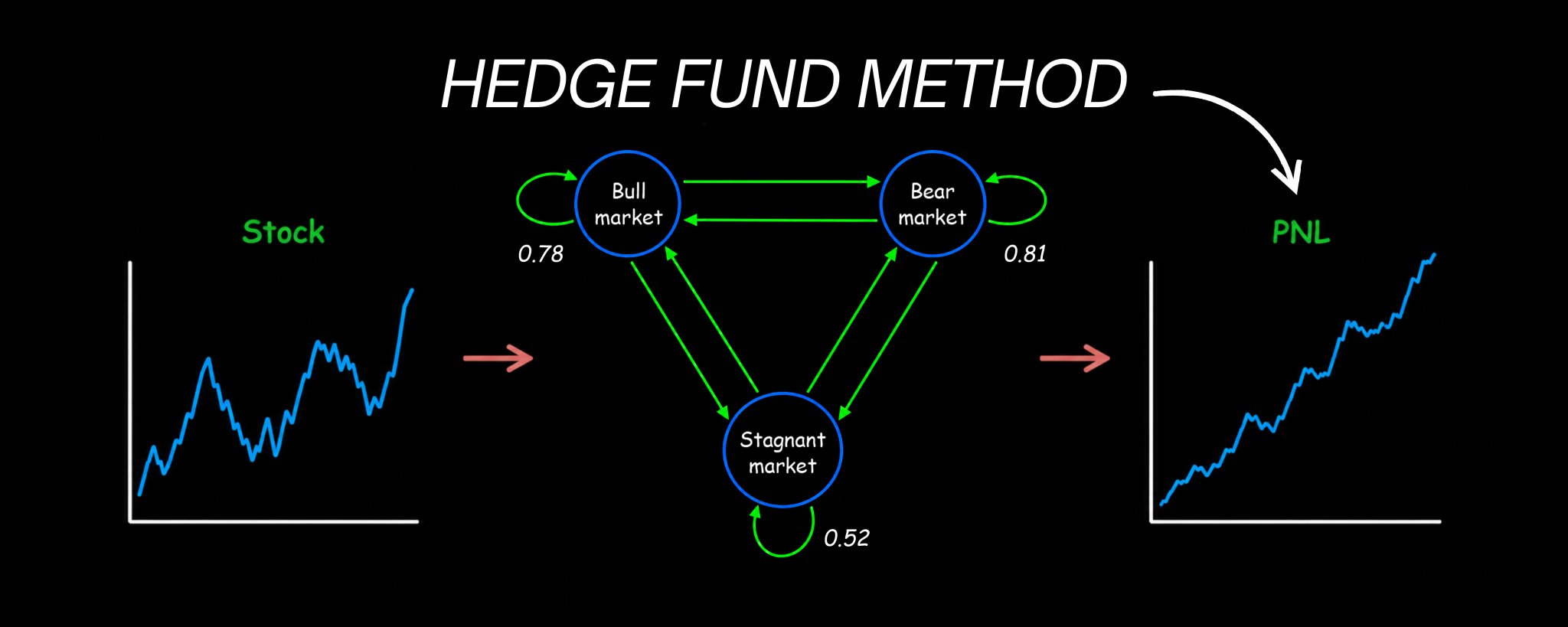
I am going to break down how hedge funds use Markov Chains to find high probability winning trades consistently & share the exact framework you can start building today. Let’s get straight to it.
Bookmark This - I’m Roan, a backend developer working on system design, HFT-style execution, and quantitative trading systems. My work focuses on how prediction markets actually behave under load. For any suggestions, thoughtful collaborations, partnerships DMs are open.
Most traders look at a chart and see price.
Quants look at the same chart and see something completely different. They see a sequence of states. Bull. Bear. Sideways. Each state carrying its own probability of persisting or transitioning into the next one. Each transition governed by mathematics that has been used to model everything from loan defaults to DNA sequences to Google’s original PageRank algorithm.
The framework is called a Markov Chain. And it is one of the most versatile and underused tools in systematic trading.
While most retail traders are drawing support lines and watching RSI, the quantitative research teams at firms like Citadel and Two Sigma are building regime-switching models that understand not just where the market is, but where it is most likely to go next based on where it has been. The math behind those models starts exactly here.
I have already written the complete neural networks implementation framework for building machine learning trading signals. That article is the next logical companion to this one.
May 6
By the end of this article you will understand exactly what a Markov Chain is and why it maps market behavior better than any single indicator, how to build a complete state transition model from real market data, how to compute the probability of any future market state using nothing more than matrix multiplication, the complete implementation pipeline from raw price data to live trading signals, and the exact mistakes that cause most Markov Chain models to fail in live markets.
Note: This article is deliberately long. Every part builds on the one before it. If you are serious about adding a genuine quantitative edge to your trading, read every single word. If you are looking for a shortcut, this is not for you.
Part 1: Why Independence Fails and Where Markov Chains Begin
Before you can build anything with Markov Chains, you need to understand the fundamental problem they were designed to solve.
Most basic probability models assume independence. Each event is treated as though it has no connection to what came before it. Roll a die. The outcome of roll 100 has nothing to do with roll 99. Each roll is completely independent.
Markets do not work this way.
Imagine you are modeling a portfolio of loans. Each loan at any point in time can be in one of four states: current, 30 to 59 days late, 60 to 89 days late, or 90 plus days late. You want to model how this portfolio evolves over time. So you try the simplest approach. You model each month independently. You draw from each state’s historical distribution.
One month later, your model says that some loans that were current last month are now 90 plus days delinquent.
That is mathematically impossible. A loan cannot jump from current to 90 plus days late in a single 30-day period. The naive independence assumption produced a model that violates reality.
This is exactly the problem Markov Chains solve. Instead of assuming each step is independent of everything that came before it, a Markov Chain introduces local conditional dependence. The next state depends on the current state. Not on everything that happened ten steps ago. Just on where you are right now.
Formally, a sequence of random variables X₀, X₁, X₂, … is a Markov Chain if it satisfies the Markov property:
P(Xₙ₊₁ = s | X₀, X₁, …, Xₙ) = P(Xₙ₊₁ = s | Xₙ)
The probability of the next state depends only on the current state, not on the entire history. This single property is what makes Markov Chains simultaneously tractable and powerful. They capture the essential dependency structure of a process without requiring you to track the entire history.
For financial markets, this translates directly. The probability that the market will be in a bull regime next month depends on whether it is in a bull, bear, or sideways regime this month. Not on what happened two years ago. The current state carries all the relevant information you need to forecast the next state.
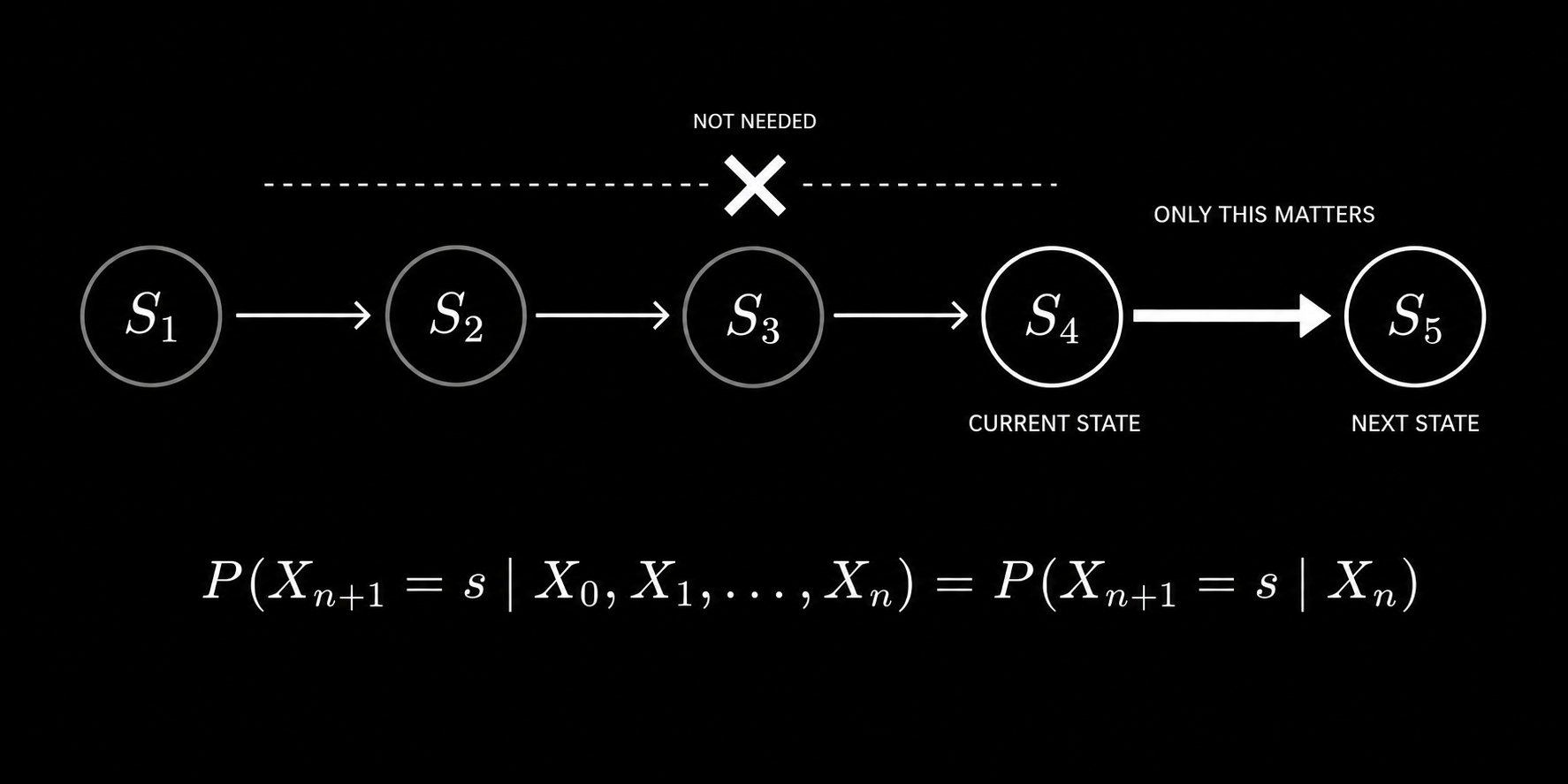
The Markov property states that the probability of the next state depends only on the current state, not on the full history of past states.
This is not a simplification made for convenience. It is a mathematically principled assumption that, when applied correctly, produces models that are dramatically more accurate than naive independence while remaining computationally tractable.
Part 2: Building the State Space and Transition Matrix
The first practical step in building a Markov Chain trading model is defining your states. This is more important than most practitioners realize.
For financial markets, common state definitions include:
Volatility regimes: Low volatility, medium volatility, high volatility defined by rolling realized volatility thresholds. Trend regimes: Bull, bear, sideways defined by the position of price relative to moving averages or by the sign and magnitude of recent returns. Liquidity regimes: High liquidity, low liquidity defined by bid-ask spreads or order book depth. Credit regimes: Risk-on, risk-off defined by credit spreads or cross-asset correlations.
For a concrete starting implementation, a three-state market regime model works well. Define:
State 0 as Bull: the 20-day return is above a positive threshold. State 1 as Bear: the 20-day return is below a negative threshold. State 2 as Sideways: everything in between.
The key requirement is that your states must be mutually exclusive and collectively exhaustive. Every observation must fall into exactly one state at any point in time. No gaps and no overlaps.
Once you have defined your states, you need to estimate the transition probabilities between them. This is the transition matrix. Each entry P(i,j) represents the probability of moving from state i to state j in one time step.
The transition matrix for a three-state model looks like this:
P = | P(0,0) P(0,1) P(0,2) | | P(1,0) P(1,1) P(1,2) | | P(2,0) P(2,1) P(2,2) |
Each row must sum to exactly 1.0 because from any given state, the system must transition to some state in the next step, including staying in the same state.
The maximum likelihood estimator for each transition probability is beautifully simple. Count how many times the system transitioned from state i to state j. Divide by the total number of transitions out of state i:
P̂(i,j) = Count(i → j) / Count(i → any state)
This is exactly how you would intuitively estimate a probability. It is also what the full derivation of the maximum likelihood estimator produces when you maximize the log-likelihood function for Markov Chain data. The intuitive answer and the mathematically rigorous answer are the same.
Here is the complete Python implementation:
import numpy as np
import pandas as pd
import yfinance as yf

def define_market_states(returns, bull_threshold=0.02, bear_threshold=-0.02, window=20):
    rolling_return = returns.rolling(window).sum()
    states = np.where(rolling_return > bull_threshold, 0,
             np.where(rolling_return < bear_threshold, 1, 2))
    return pd.Series(states, index=returns.index)

def estimate_transition_matrix(states, n_states=3):
    transition_counts = np.zeros((n_states, n_states))
    state_values = states.dropna().values

    for i in range(len(state_values) - 1):
        current_state = int(state_values[i])
        next_state = int(state_values[i + 1])
        if not np.isnan(current_state) and not np.isnan(next_state):
            transition_counts[current_state][next_state] += 1

    transition_matrix = np.zeros((n_states, n_states))
    for i in range(n_states):
        row_sum = transition_counts[i].sum()
        if row_sum > 0:
            transition_matrix[i] = transition_counts[i] / row_sum

    return transition_matrix

ticker = yf.Ticker("SPY")
df = ticker.history(period="10y", interval="1d")
returns = df['Close'].pct_change().dropna()

states = define_market_states(returns)
P = estimate_transition_matrix(states)

state_names = ['Bull', 'Bear', 'Sideways']
print("Transition Matrix:")
print(pd.DataFrame(P, index=state_names, columns=state_names).round(3))
The transition matrix you produce from this process is the map of your market. Every entry tells you the probability of moving between two specific regimes. It is the foundation of everything that follows.
Part 3: Computing Multi-Step Transition Probabilities
This is where Markov Chains become genuinely powerful as a trading tool.
You now have the one-step transition matrix P. But what you really want to know as a trader is not just what happens next month. You want to know what the market is likely to look like in three months, six months, twelve months. You want to know the probability of starting in a bull regime today and ending up in a bear regime after twelve transitions.
This is where the Chapman-Kolmogorov equation comes in. It states that the n-step transition probability from state i to state j is the (i,j) entry of the matrix P raised to the nth power:
P^(n)(i,j) = [Pⁿ]ᵢⱼ
That is it. To compute the probability of transitioning from any state to any other state in n steps, you simply multiply the transition matrix by itself n times and read the corresponding entry.
This is an extraordinarily elegant result. All the mathematical complexity of computing paths through a state space over multiple steps reduces to a single matrix power.
def multi_step_transition(P, n_steps):
    return np.linalg.matrix_power(P, n_steps)

def regime_probability_forecast(P, current_state, n_steps, state_names):
    P_n = multi_step_transition(P, n_steps)
    probabilities = P_n[current_state]

    print(f"\nFrom {state_names[current_state]} regime:")
    print(f"After {n_steps} steps:")
    for i, (name, prob) in enumerate(zip(state_names, probabilities)):
        print(f"  Probability of {name}: {prob:.4f}")

    return probabilities

state_names = ['Bull', 'Bear', 'Sideways']

for steps in [1, 5, 12, 24]:
    regime_probability_forecast(P, current_state=0, n_steps=steps, state_names=state_names)
What this tells you as a trader is specific and actionable. If you are currently in a bull regime, you can now quantify the probability that you will still be in a bull regime in 12 months versus having transitioned to bear or sideways. That probability informs your position sizing, your hedging decisions, and your strategy allocation.
There is another critical output from this framework: the stationary distribution. As n becomes very large, the distribution across states converges to a fixed vector π regardless of the starting state:
π = π × P
The stationary distribution tells you the long-run proportion of time the market spends in each regime. In practice, you solve for π using:
def find_stationary_distribution(P):
    n = P.shape[0]
    A = (P.T - np.eye(n))
    A[-1] = 1
    b = np.zeros(n)
    b[-1] = 1

    pi = np.linalg.solve(A, b)
    return pi

pi = find_stationary_distribution(P)
state_names = ['Bull', 'Bear', 'Sideways']
print("\nStationary Distribution:")
for name, prob in zip(state_names, pi):
    print(f"  {name}: {prob:.4f}")
The stationary distribution is your long-run baseline. Any strategy that bets heavily on a regime that the stationary distribution tells you is rare is taking on significant tail risk. Knowing the long-run regime proportions is essential for strategy design.
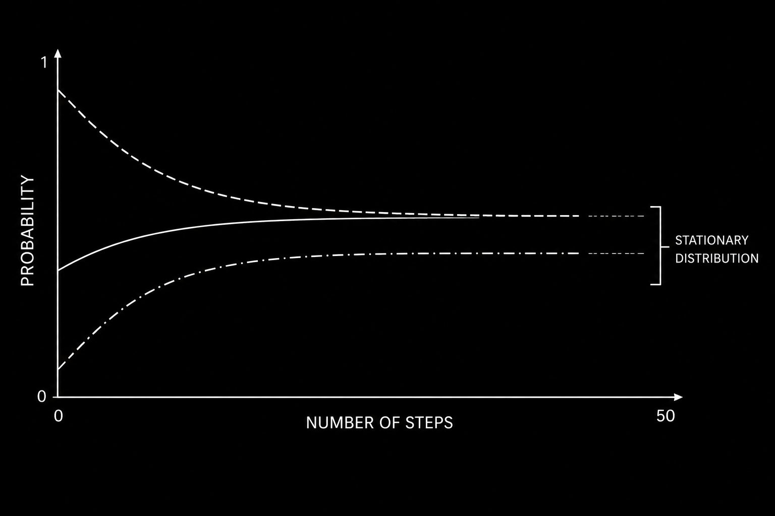
Regardless of starting state, the probability distribution across regimes converges to a fixed stationary distribution as the number of steps increases.
Part 4: From Regime Model to Trading Signal
Having a regime model is not a trading strategy. Converting it into one requires connecting the regime probabilities to specific position decisions.
The core insight is this: the Markov Chain gives you a probability distribution over future states at each point in time. Your trading signal is a function of that distribution.
The simplest approach is direct regime-based allocation. When the model says you are in a bull regime, go long. When bear, go short or flat. When sideways, reduce position size.
A more sophisticated approach uses the full probability vector as input to position sizing. The current state distribution vector π_t represents your probability allocation across regimes at time t. You can construct a position that is proportional to your confidence in each regime:
def compute_trading_signal(current_state, P, strategy_returns_by_regime):
    one_step = P[current_state]

    bull_prob = one_step[0]
    bear_prob = one_step[1]
    sideways_prob = one_step[2]

    signal = bull_prob - bear_prob

    if signal > 0.3:
        position = 1.0
    elif signal < -0.3:
        position = -1.0
    elif abs(signal) < 0.1:
        position = 0.0
    else:
        position = signal / 0.3

    return position, one_step

def backtest_markov_strategy(returns, states, P, lookback=252):
    positions = []
    dates = []

    state_values = states.dropna()

    for i in range(lookback, len(state_values)):
        historical_states = state_values.iloc[i-lookback:i]
        P_estimated = estimate_transition_matrix(historical_states)

        current_state = int(state_values.iloc[i])
        position, probs = compute_trading_signal(current_state, P_estimated, None)

        positions.append(position)
        dates.append(state_values.index[i])

    positions_series = pd.Series(positions, index=dates)
    strategy_returns = positions_series.shift(1) * returns.loc[dates]

    sharpe = strategy_returns.mean() / strategy_returns.std() * np.sqrt(252)

    cumulative = (1 + strategy_returns).cumprod()
    rolling_max = cumulative.cummax()
    max_drawdown = ((cumulative - rolling_max) / rolling_max).min()

    print(f"Annualized Sharpe: {sharpe:.4f}")
    print(f"Maximum Drawdown: {max_drawdown:.4f}")
    print(f"Annual Return: {strategy_returns.mean() * 252:.4f}")

    return strategy_returns, positions_series
The walk-forward structure in the backtest above is critical. You re-estimate the transition matrix at each step using only the historical data available at that point. You never use future information to estimate past probabilities. This is the difference between a realistic backtest and one that is guaranteed to disappoint in live trading.
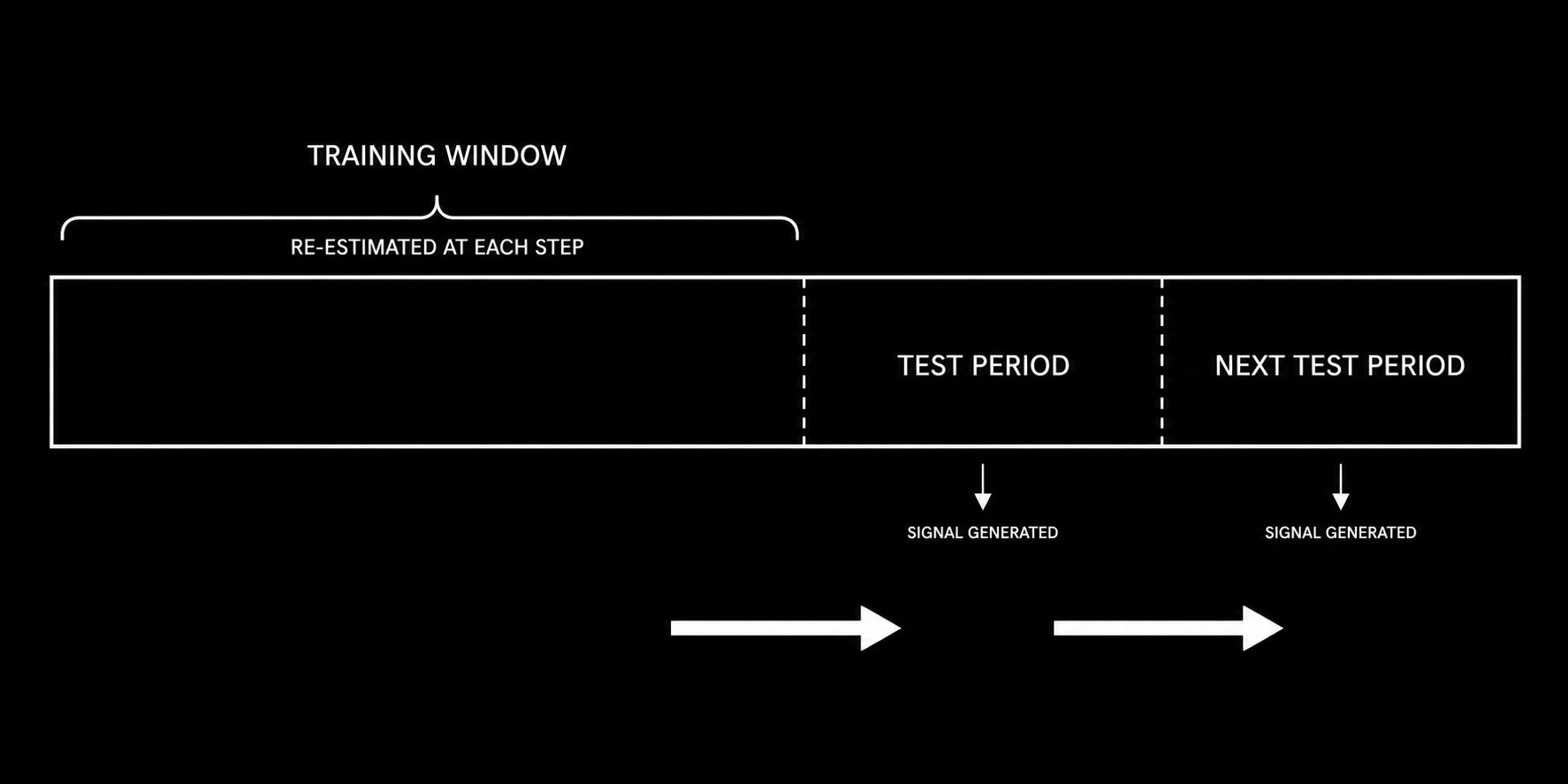
The walk-forward structure ensures the transition matrix is estimated only from data available at each point in time, preventing lookahead bias.
Part 5: The Complete Implementation Pipeline and Critical Limitations
This section assembles everything into a production-ready Markov Chain trading system and addresses the assumptions that will determine whether your model survives contact with live markets.
Complete system implementation:
import numpy as np
import pandas as pd
import yfinance as yf
from sklearn.preprocessing import StandardScaler
import warnings
warnings.filterwarnings('ignore')

class MarkovChainTradingSystem:
    def __init__(self, n_states=3, lookback_window=252, regime_window=20):
        self.n_states = n_states
        self.lookback_window = lookback_window
        self.regime_window = regime_window
        self.transition_matrix = None
        self.state_names = ['Bull', 'Bear', 'Sideways']

    def fetch_data(self, ticker, period="10y"):
        data = yf.Ticker(ticker).history(period=period, interval="1d")
        self.returns = data['Close'].pct_change().dropna()
        self.prices = data['Close']
        return self.returns

    def label_states(self, returns, bull_thresh=0.02, bear_thresh=-0.02):
        rolling_ret = returns.rolling(self.regime_window).sum()
        states = np.where(rolling_ret > bull_thresh, 0,
                 np.where(rolling_ret < bear_thresh, 1, 2))
        return pd.Series(states, index=returns.index)

    def estimate_transition_matrix(self, states):
        counts = np.zeros((self.n_states, self.n_states))
        vals = states.dropna().values.astype(int)
        for i in range(len(vals) - 1):
            if 0 <= vals[i] < self.n_states and 0 <= vals[i+1] < self.n_states:
                counts[vals[i]][vals[i+1]] += 1
        P = np.zeros_like(counts)
        for i in range(self.n_states):
            if counts[i].sum() > 0:
                P[i] = counts[i] / counts[i].sum()
        return P

    def stationary_distribution(self, P):
        n = P.shape[0]
        A = (P.T - np.eye(n))
        A[-1] = 1
        b = np.zeros(n)
        b[-1] = 1
        try:
            return np.linalg.solve(A, b)
        except:
            return np.ones(n) / n

    def generate_signal(self, P, current_state):
        probs = P[current_state]
        return probs[0] - probs[1]

    def run_walkforward_backtest(self):
        states = self.label_states(self.returns)
        signals = []

        for i in range(self.lookback_window, len(states)):
            historical = states.iloc[i - self.lookback_window:i]
            P = self.estimate_transition_matrix(historical)
            current = int(states.iloc[i])
            signal = self.generate_signal(P, current)
            signals.append({'date': states.index[i], 'signal': signal,
                           'state': self.state_names[current]})

        signals_df = pd.DataFrame(signals).set_index('date')
        position = np.sign(signals_df['signal'])
        position[abs(signals_df['signal']) < 0.1] = 0

        strategy_returns = position.shift(1) * self.returns.loc[signals_df.index]

        sharpe = strategy_returns.mean() / strategy_returns.std() * np.sqrt(252)
        cumulative = (1 + strategy_returns).cumprod()
        max_dd = ((cumulative - cumulative.cummax()) / cumulative.cummax()).min()

        print(f"\nMarkov Chain Trading System Results:")
        print(f"Annualized Sharpe Ratio: {sharpe:.4f}")
        print(f"Maximum Drawdown: {max_dd:.4f}")
        print(f"Annualized Return: {strategy_returns.mean() * 252:.4f}")
        print(f"\nRegime Distribution:")
        print(signals_df['state'].value_counts(normalize=True).round(3))

        return strategy_returns, signals_df

system = MarkovChainTradingSystem()
system.fetch_data("SPY")
returns, signals = system.run_walkforward_backtest()
The three assumptions you must understand before deploying:
The first is the Markov property itself. The model assumes that the next state depends only on the current state, not on longer history. In reality, markets sometimes exhibit longer-range dependencies. A trend that has been running for six months may have different transition probabilities than one that just started. You can partially address this by expanding your state space to include duration information, though this increases complexity significantly.
The second is time homogeneity. The model assumes transition probabilities are constant over time. They are not. The probability of a bull regime transitioning to bear was very different in 2008 than in 2021. The standard mitigation is rolling window re-estimation, which you have already seen in the walk-forward backtest above. Shorter windows adapt faster but produce noisier estimates. Longer windows produce more stable estimates but lag regime changes.
The third is sufficient data for reliable estimation. The maximum likelihood estimator converges to true transition probabilities as you observe more transitions. With few observations, particularly for rare transitions, your estimates will be noisy and unreliable. Always check that every cell in your transition matrix has been estimated from at least 20 to 30 observed transitions. If not, consider merging states or extending your data history.
Part 6: Hidden Markov Models - Taking the Framework Further
Every assumption in the model so far has one thing in common. You assumed you could see the regime.
You labeled each day as Bull, Bear, or Sideways using rolling returns. But the regime was never directly observable. You reverse engineered it from price. That is not the same thing. A bear regime that has not yet shown up in prices because institutional positioning is quietly shifting beneath the surface is completely invisible to your state labels. This is the core limitation of observable Markov Chains. Hidden Markov Models fix it.
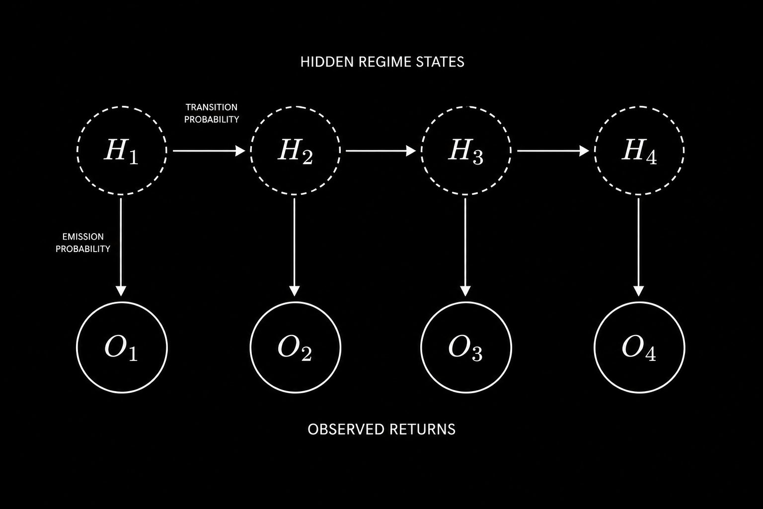
In a Hidden Markov Model, the true market regime is unobservable. Only noisy return observations are available, from which the hidden regime sequence must be inferred.
In an HMM, the true regime is a hidden state you cannot observe. What you can observe is the returns sequence. Each hidden state generates returns from its own distribution. The bull regime produces returns with a positive mean and low variance. The bear regime produces returns with a negative mean and high variance. The model learns both the regime transitions and the return distributions at the same time, from price data alone, without you ever labeling a single day by hand.
There are two algorithms that make this work.
The first is Baum-Welch. This is the algorithm that estimates all model parameters from the observable return sequence. You give it returns. It learns the transition matrix, the return distribution for each regime, and the starting probabilities, all without requiring labeled data. It runs forward through the sequence computing probabilities, then backward to refine them, repeating until convergence.
The second is Viterbi. Once you have a fitted model, Viterbi decodes the most likely sequence of hidden regimes that produced your observed returns. It does not give you soft probabilities. It gives you the single best path through the hidden state space.
from hmmlearn import hmm
import numpy as np
import pandas as pd

def fit_market_hmm(returns, n_states=3, n_iter=1000):
    X = returns.values.reshape(-1, 1)

    model = hmm.GaussianHMM(
        n_components=n_states,
        covariance_type="full",
        n_iter=n_iter,
        random_state=42
    )
    model.fit(X)

    hidden_states = model.predict(X)

    state_means = {s: returns[hidden_states == s].mean() for s in range(n_states)}
    sorted_states = sorted(state_means, key=state_means.get, reverse=True)
    state_map = {old: new for new, old in enumerate(sorted_states)}
    labeled = np.array([state_map[s] for s in hidden_states])

    print("Learned Transition Matrix:")
    print(np.round(model.transmat_, 3))

    state_names = ['Bull', 'Bear', 'Sideways']
    for i in range(n_states):
        mask = labeled == i
        print(f"{state_names[i]}: mean={returns[mask].mean():.4f}, vol={returns[mask].std():.4f}")

    return model, labeled

model, labeled_states = fit_market_hmm(returns)
The signal generation is identical to Part 4. At each step you compute the probability of being in each regime right now. You multiply that vector by the transition matrix to get the one step ahead forecast. Bull probability minus bear probability gives your position.
def hmm_signal(model, returns, lookback=252):
    signals = []

    for i in range(lookback, len(returns)):
        window = returns.iloc[i - lookback:i].values.reshape(-1, 1)
        posteriors = model.predict_proba(window)
        current_probs = posteriors[-1]
        next_probs = current_probs @ model.transmat_
        signals.append(next_probs[0] - next_probs[1])

    return pd.Series(signals, index=returns.index[lookback:])
Two things to keep in mind before you deploy this. Baum-Welch finds a local maximum, not a global one. Always run it from multiple random starts and keep the model with the highest log likelihood. The default single initialization will frequently produce suboptimal regime assignments. The emission variables you choose matter more than any other design decision. Returns alone carry limited information about the true economic regime. Returns combined with realized volatility, credit spreads, and VIX term structure give the model a much richer signal. The choice of what to feed as observations is where domain knowledge compounds the mathematics.
The observable Markov Chain gave you a regime map. The Hidden Markov Model builds that map in real time from noisy signals, without requiring a single manually labeled data point. That is the direction institutional regime switching models have moved. You now have the complete framework to build one.
The Summary
Markov Chains do not predict the future. What they do is something more useful. They quantify the probability of every possible future state given the current state. They give you a mathematical map of market regimes and the likelihood of transitioning between them.
The framework is fully implementable in a weekend. The transition matrix is estimated from historical data in a handful of lines of Python. The Chapman-Kolmogorov equation gives you n-step forecasts through a single matrix power. The stationary distribution tells you the long-run baseline. And the walk-forward backtest tells you whether your model has genuine predictive power or is fitting noise.
The assumptions are real and they matter. Time homogeneity is violated. The Markov property is an approximation. Estimation error is always present. But as a first pass model and as a building block for more sophisticated Hidden Markov Model extensions, this framework has been deployed in production at real firms and has generated real edge.
You now have the complete implementation. The code is in this article. The mathematics is explained from first principles. The critical limitations are documented so you know exactly where the model can fail and how to mitigate those failures.
Here is the question I want you to sit with.
The Markov Chain model defines regimes based on observable price behavior. But the most important market regimes, the ones that institutional traders actually trade around, are often driven by latent factors like credit conditions, monetary policy stance, and risk appetite that are not directly visible in price data alone. If you were designing a Hidden Markov Model for markets, what observable signals would you use as your emission variables and why?
Drop your answer in the comments.
There is no wrong answer but there are very revealing ones.
Source
Written by @RohOnChain · View original post · Published: 2026-05-06
Neural Networks — ML Signal Framework
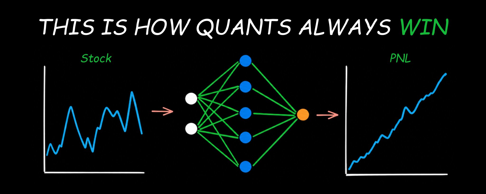
I am going to break down how hedge funds use neural networks to extract edge before the trade even happens & share the exact implementation framework you can build today. Let’s get straight to it.
Bookmark This - I’m Roan, a backend developer working on system design, HFT-style execution, and quantitative trading systems. My work focuses on how prediction markets actually behave under load. For any suggestions, thoughtful collaborations, partnerships DMs are open.
The way most traders lose money has nothing to do with their market thesis. They are right about direction more often than they think. The problem is they are operating on one signal, one indicator, one gut feeling. They are making probability decisions without a probability framework. And markets punish that mistake reliably and repeatedly. Neural networks solve a fundamentally different problem. They do not predict the future. What they do is learn the expectation function hidden inside historical data. The mathematical relationship between what you can observe right now and what the market is statistically most likely to do next. And they do this across thousands of variables simultaneously in ways no human eye can see and no single indicator can capture.
The largest funds already know this. Two Sigma runs over 10,000 live signals through machine learning models simultaneously. Citadel’s quantitative research division deploys deep learning architectures across equity, options, and macro strategies. Renaissance Technologies built the Medallion Fund entirely on this framework decades before anyone else understood what they were doing. The fund returned 66 percent annually before fees over 30 years. That is not luck. That is the systematic application of statistical learning at scale.
The entry level quant researcher building these models at those firms earns between $350,000 and $650,000 in total compensation. Not because the job is glamorous. Because finding a reliable edge in financial data using mathematics is genuinely one of the hardest unsolved problems in applied science.
If you have not yet read the complete quant roadmap covering the mathematical foundation underneath everything in this article, start there first.
Apr 28
AI and machine learning hiring in quantitative finance accelerated sharply through 2025. Every major systematic fund is building signal generation infrastructure powered by deep learning. And yet most traders who try to implement neural networks into their strategy fail at the same predictable step for the same predictable reason.
This article tells you exactly what that step is and exactly how to avoid it. Then it gives you the complete implementation framework from data preparation through live signal deployment.
By the end of this article you will understand exactly how neural networks learn from data and what they are actually computing when they make a prediction, why applying them directly to price charts is guaranteed to fail and what the correct input is, which architecture works best for sequential market data and why, the complete rigorous training framework that separates real edge from self-deception and the full implementation pipeline to deploy your first neural network trading signal.
Note: This article is deliberately long. Every part builds on the one before it. If you are serious about adding a genuine quantitative edge to your trading, read every single word. If you are looking for a shortcut, this is not for you.
Part 1: What a Neural Network Actually Computes
Before you build anything, you need to understand what is actually happening when a neural network trains on data. Most explanations skip this and go straight to code. That is why most implementations fail.
A neural network is a parameterized composite function. You give it a vector of inputs. It applies a sequence of linear transformations interleaved with non-linear activation functions. It produces an output. The formal structure is:
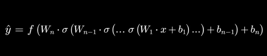
Where W_i are weight matrices, b_i are bias vectors, and σ is a non-linear activation function applied element-wise. This is the mathematical reality underneath every neural network regardless of how it is visualized.
The power is in training. You have a dataset of input-output pairs. The network starts with random parameters. It makes a prediction. It computes the error between that prediction and the actual observed output. It adjusts the parameters in the direction that reduces the error. It repeats this millions of times.
The formal objective is minimizing a loss function. For regression tasks the standard choice is mean squared error:
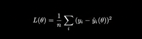
Where θ represents all learnable parameters, yᵢ is the actual observed value, and ŷᵢ is the model prediction. The optimization proceeds by computing the gradient of the loss with respect to the parameters and taking a step in the negative gradient direction: θ ← θ - α · ∇_θ L(θ) Where α is the learning rate. This is stochastic gradient descent. Every modern deep learning optimizer is a variation of this with adaptive step sizes, momentum terms, or second-order approximations layered on top.
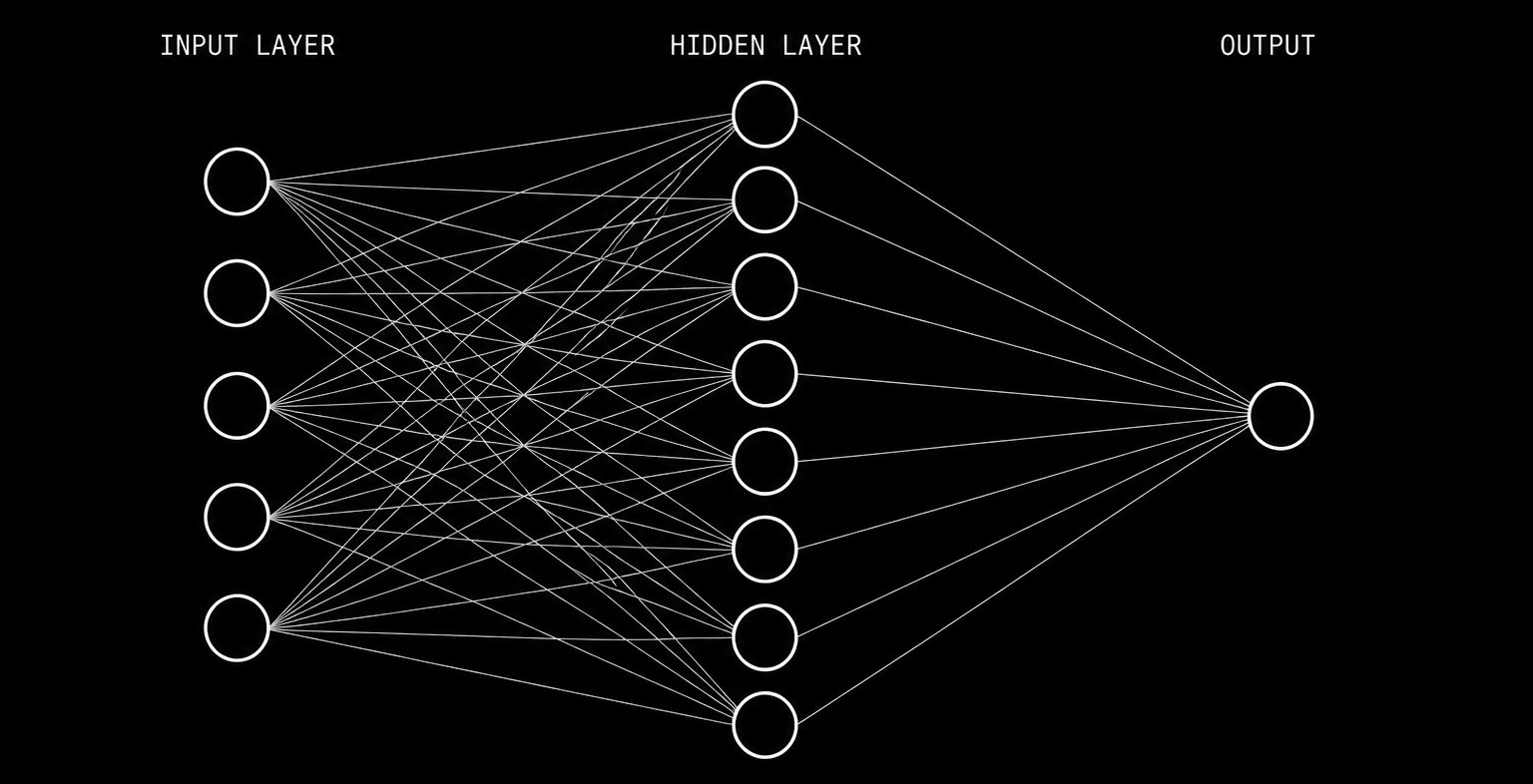
A feedforward neural network passes inputs through weighted layers to produce an output that approximates the conditional expectation of the target variable.
Now here is the insight that changes how you interpret everything a neural network produces.
When you train a network to minimize squared error against a target variable, what does it learn? It learns the conditional expectation of that variable given your inputs. The function that minimizes E[(Y - f(X))²] is exactly E[Y|X]. This is not a prediction in the colloquial sense. It is a mathematical expectation. The weighted average outcome across all scenarios consistent with the observed inputs.
The proof of this is straightforward. Expand the squared loss:
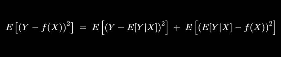
The first term is irreducible variance. The second term is minimized by setting f(X) = E[Y|X]. The optimal predictor under squared error is the conditional mean.
This has a profound practical implication. When you roll a fair die 10,000 times and train a neural network to minimize squared error against the outcomes, it will predict 3.5. Can a die land on 3.5? No. But 3.5 is the value that minimizes the expected squared error. The network is computing the expectation, not the next realization.
Why does neural networks specifically outperform simpler models at learning this conditional expectation? The universal approximation theorem. A feedforward network with a single hidden layer containing sufficient neurons can approximate any continuous function on a compact subset of Rⁿ to arbitrary precision. For deep networks with multiple layers, the approximation becomes exponentially more efficient in terms of the number of parameters required.
This means: if there is any smooth mathematical relationship between your input features and your target variable, a properly architected neural network can find it. The question is never whether the network can learn the function. The question is whether the function you want it to learn is actually stable enough across time to be worth learning.
Part 2: Why Price Prediction Fails and What to Do Instead
This is the most important section in the article. The mistake described here is made by virtually every trader who tries to implement neural networks for the first time. Understanding why it fails is the prerequisite for everything that works.
The failure mode is this: take 500 days of closing prices, feed them into an LSTM, ask it to predict day 501.
In-sample, the predictions look smooth and close to actual prices. Out-of-sample, the model predicts something roughly constant or reverts to a recent mean while prices move somewhere completely different. The model appears to have learned nothing useful.
This is not a model failure. It is a data distribution failure.
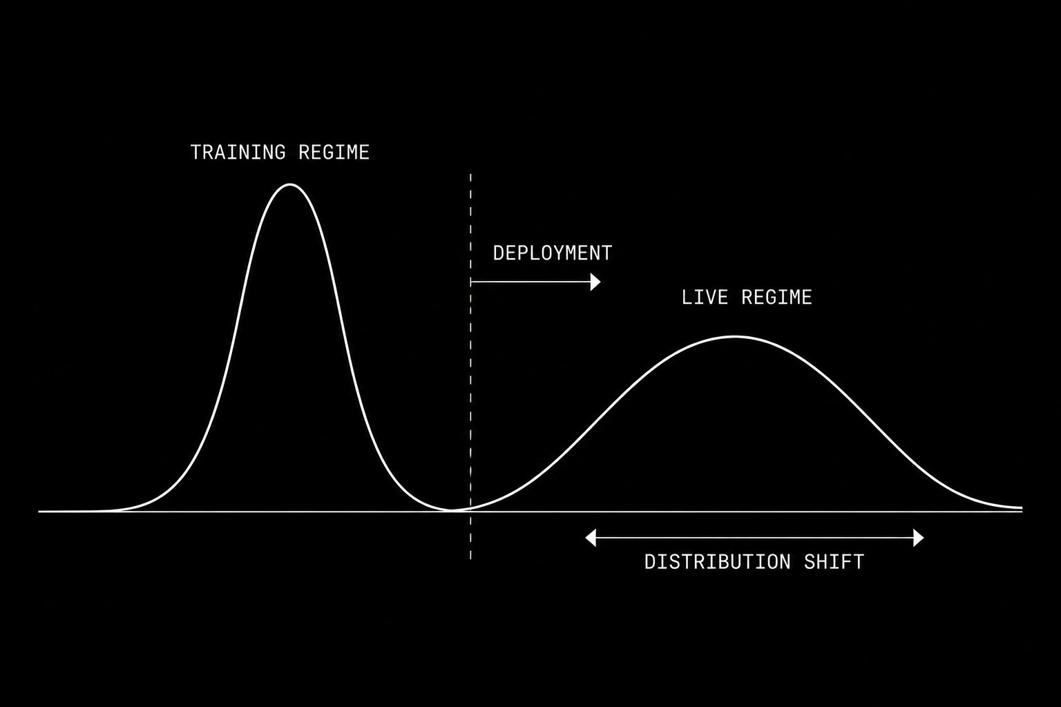
The distribution governing market returns shifts continuously over time. A model trained on the left regime learns the wrong expectation function for the right regime.
Recall from Part 1: a neural network learns E[Y|X], the conditional expectation of Y given X. This expectation is only meaningful if the data generating distribution P(Y|X) is stable over time. If that distribution shifts, the conditional expectation the model learned from historical data no longer describes the expectation in the present.
Formally, this is the problem of non-stationarity. A time series {Xₜ} is stationary if its joint distribution P(Xₜ₁, Xₜ₂, …, Xₜₙ) is invariant to time shifts. Financial price series are non-stationary in the strongest possible sense. The distribution governing equity returns in 2008 is structurally different from the distribution governing them in 2021. Mean, variance, autocorrelation, and tail behavior all shift as a function of regime, liquidity, volatility clustering, and macro conditions.
The consequence is visible in any backtest of a price-predicting neural network. The model trained on 2015 to 2019 data learns the expectation structure of that regime. When the distribution shifts in 2020, the model is fitting a moving target. Its predictions are always wrong in a systematic way that reveals it is modeling the past distribution, not the present one.
What is the solution?
Feature engineering to produce stationary or near-stationary inputs. The target variable itself should also be constructed to be approximately stationary.
For inputs, the features that have exhibited reasonable stationarity across market regimes include:
Log returns over multiple windows: r_t = ln(P_t / P_{t-k}) for k in {1, 5, 20}
Volatility ratios: σ_short / σ_long where each σ is rolling realized volatility over different windows
Momentum signals normalized by volatility: r_t / σ_t, the return scaled by realized risk
Volume z-score: (V_t - μ_V) / σ_V computed over a rolling window
Spread-based signals: bid-ask spread relative to its historical distribution, or effective spread computed from trade price versus midpoint
Regime indicators: VWAP deviation, distance from rolling high and low, implied versus realized volatility ratio
For the target variable, instead of predicting next period price, predict next period direction as a binary classification problem: will the risk-adjusted return be positive? Or predict next period return z-scored against its recent distribution. Both targets are more stable than raw price or even raw return.
The practical test for whether a feature is useful: run an augmented Dickey-Fuller test on it. A p-value below 0.05 suggests the series is stationary. For features that fail this test, first-difference them or normalize by a rolling standard deviation.
Implementation note: In Python, this looks like:
from statsmodels.tsa.stattools import adfuller
import numpy as np

def check_stationarity(series, name):
    result = adfuller(series.dropna())
    print(f"{name}: ADF statistic={result[0]:.4f}, p-value={result[1]:.4f}")
    return result[1] < 0.05

**Example: Feature Engineering**
returns = df['close'].pct_change()
vol_20 = returns.rolling(20).std()
vol_5 = returns.rolling(5).std()

features = {
    'return_1d': returns,
    'return_5d': df['close'].pct_change(5),
    'vol_ratio': vol_5 / vol_20,
    'momentum': returns / vol_20,
    'volume_zscore': (df['volume'] - df['volume'].rolling(20).mean()) / df['volume'].rolling(20).std()
}

for name, series in features.items():
    is_stationary = check_stationarity(series, name)
Every feature that fails the stationarity test is a feature that will cause your model to learn the wrong distribution.
Part 3: The LSTM Architecture for Sequential Market Data
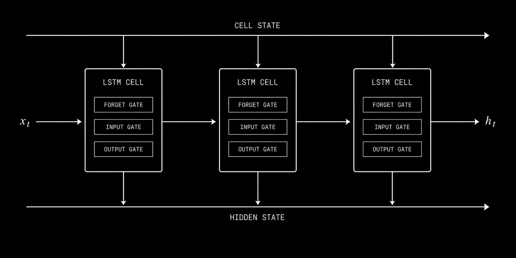
The LSTM forget gate, input gate, and output gate control what information persists across time steps, allowing the model to maintain context across weeks of market data.
Market data is sequential. The order of events carries information that a snapshot does not. What happened in the last five minutes is connected to what happens in the next five minutes through autocorrelation, momentum, mean reversion, and microstructure dynamics. The architecture you use must be capable of learning from this sequential structure.
A standard feedforward network treats every input independently. When you present it with day 100’s feature vector, it has no knowledge of what days 1 through 99 looked like. For non-sequential data like the football throwing example from Part 1, this is fine. For time series data from financial markets, it throws away the most important information in your dataset.
The Recurrent Neural Network addresses this by passing a hidden state forward through time. At each time step t, the hidden state h_t is computed as:
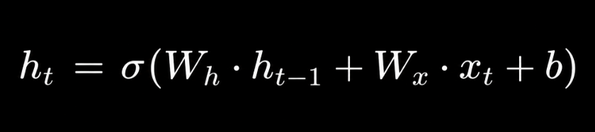
The hidden state encodes everything the network has learned from steps 1 through t-1 and combines it with the current input x_t. This is the memory mechanism. But basic RNNs suffer from the vanishing gradient problem: gradients diminish exponentially as they are backpropagated through time, making it effectively impossible to learn dependencies across more than a few time steps.
LSTM solves this with a gated memory architecture. Rather than a single hidden state, the LSTM maintains both a hidden state h_t and a cell state c_t. The cell state is the long-term memory. The hidden state is the working memory. Three learned gates control information flow:
Forget gate: f_t = σ(W_f · [h_{t-1}, x_t] + b_f) This gate decides what fraction of the previous cell state to discard. When markets transition between regimes, the forget gate allows the model to release outdated patterns and reset its understanding.
Input gate: i_t = σ(W_i · [h_{t-1}, x_t] + b_i), g_t = tanh(W_g · [h_{t-1}, x_t] + b_g) These gates decide what new information to write into the cell state.
Output gate: o_t = σ(W_o · [h_{t-1}, x_t] + b_o), h_t = o_t ⊙ tanh(c_t) This gate decides what to output from the cell state.
The cell state update combines forgetting and new writing: c_t = f_t ⊙ c_{t-1} + i_t ⊙ g_t
This architecture allows LSTM to maintain relevant context across sequences of 50, 100, or more time steps without the gradient vanishing problem. For daily trading strategies, this means the model can learn that a particular pattern of volatility compression three weeks ago predicts a specific type of breakout behavior today. No indicator-based system can capture relationships at that complexity.
Complete LSTM implementation in PyTorch:
import torch
import torch.nn as nn
import numpy as np
from sklearn.preprocessing import StandardScaler

class TradingLSTM(nn.Module):
    def __init__(self, input_size, hidden_size=64, num_layers=2, dropout=0.2):
        super(TradingLSTM, self).__init__()
        self.hidden_size = hidden_size
        self.num_layers = num_layers

        self.lstm = nn.LSTM(
            input_size=input_size,
            hidden_size=hidden_size,
            num_layers=num_layers,
            dropout=dropout,
            batch_first=True
        )

        self.dropout = nn.Dropout(dropout)
        self.fc = nn.Linear(hidden_size, 1)
        self.sigmoid = nn.Sigmoid()

    def forward(self, x):
        h0 = torch.zeros(self.num_layers, x.size(0), self.hidden_size)
        c0 = torch.zeros(self.num_layers, x.size(0), self.hidden_size)

        out, _ = self.lstm(x, (h0, c0))
        out = self.dropout(out[:, -1, :])
        out = self.fc(out)
        return self.sigmoid(out)

def prepare_sequences(features, target, lookback=10):
    X, y = [], []
    for i in range(len(features) - lookback):
        X.append(features[i:i+lookback])
        y.append(target[i+lookback])
    return np.array(X), np.array(y)
The lookback period is a critical hyperparameter. For daily strategies, start with a window of 10 to 20 trading days. For intraday strategies operating on 5-minute bars, a lookback of 24 periods covers two trading hours of context. The optimal lookback depends on the timescale of the patterns you are trying to capture and must be determined empirically through validation performance.
Part 4: Training Without Fooling Yourself
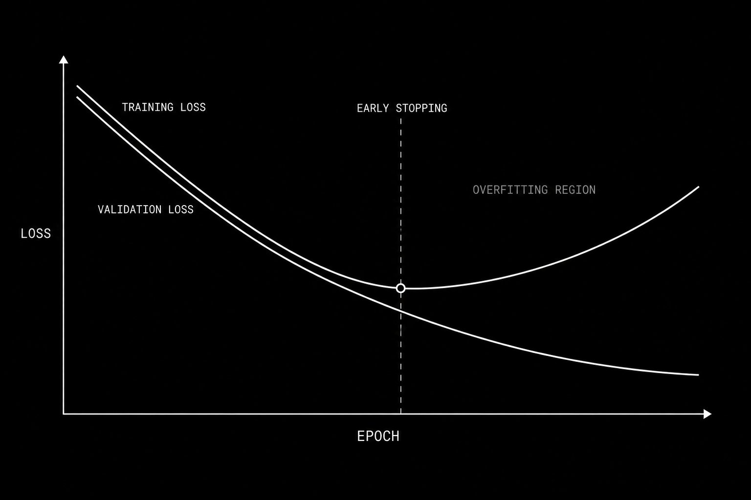
When training loss continues falling while validation loss rises, the model has crossed into overfitting. Early stopping saves the weights at the validation minimum.
Building the model is the easy part. The dangerous part is evaluating whether it actually learned something real versus memorizing the noise in your training data.
Overfitting is the central failure mode of machine learning in finance. An overfit model has found patterns in its training data that do not generalize. On training data it performs beautifully. On new data it performs at chance or worse. The critical problem is that overfit in-sample performance looks identical to genuine edge. You cannot distinguish them by looking at training metrics alone.
The solution is a rigorous three-way data split used in a specific sequential order.
The training set is where gradient descent runs. The model sees this data repeatedly during training and adjusts its parameters based on it. Never evaluate generalization performance on this set.
The validation set is data the model never trains on but that you monitor continuously during training. After each epoch, compute validation loss. The moment validation loss stops improving and begins increasing while training loss continues decreasing, you have found the overfitting threshold. Stop training immediately and save the model weights from the epoch with the lowest validation loss. This is early stopping and it is your primary defense against overfitting.
The test set is data the model has never influenced in any form. You use it exactly once: after all architecture decisions, all hyperparameter choices, and all feature engineering decisions have been finalized using the training and validation sets. The test set result is your honest estimate of live performance. Using the test set to make additional design decisions invalidates it.
For financial time series, these splits must be sequential. The training period comes first in time. The validation period follows. The test period is most recent. Randomizing the split would allow future information to contaminate training, a form of lookahead bias that guarantees your backtest looks better than live performance.
Complete training loop with early stopping:
def train_model(model, train_loader, val_loader, epochs=100, lr=0.001, patience=10):
    optimizer = torch.optim.Adam(model.parameters(), lr=lr)
    criterion = nn.BCELoss()
    scheduler = torch.optim.lr_scheduler.ReduceLROnPlateau(
        optimizer, patience=5, factor=0.5
    )

    best_val_loss = float('inf')
    best_weights = None
    patience_counter = 0

    for epoch in range(epochs):
        model.train()
        train_loss = 0
        for X_batch, y_batch in train_loader:
            optimizer.zero_grad()
            predictions = model(X_batch).squeeze()
            loss = criterion(predictions, y_batch)
            loss.backward()
            torch.nn.utils.clip_grad_norm_(model.parameters(), max_norm=1.0)
            optimizer.step()
            train_loss += loss.item()

        model.eval()
        val_loss = 0
        with torch.no_grad():
            for X_batch, y_batch in val_loader:
                predictions = model(X_batch).squeeze()
                loss = criterion(predictions, y_batch)
                val_loss += loss.item()

        val_loss /= len(val_loader)
        scheduler.step(val_loss)

        if val_loss < best_val_loss:
            best_val_loss = val_loss
            best_weights = model.state_dict().copy()
            patience_counter = 0
        else:
            patience_counter += 1
            if patience_counter >= patience:
                print(f"Early stopping at epoch {epoch}")
                break

    model.load_state_dict(best_weights)
    return model
Gradient clipping is included in this implementation for a specific reason. LSTM gradients can explode during training when the learned sequences are long. Clipping the gradient norm to a maximum value of 1.0 prevents this without significantly affecting convergence speed.
The most rigorous evaluation framework for trading specifically is walk-forward validation. Rather than a single train-validation-test split, you roll a training window forward through time, train, test on the immediately following period, then advance the window and repeat. The concatenated out-of-sample predictions across all windows give you a realistic estimate of how the model would have performed if deployed live at each historical point.
Walk-forward validation:
def walk_forward_validation(features, target, train_size, test_size, step):
    all_predictions = []
    all_actuals = []

    for start in range(0, len(features) - train_size - test_size, step):
        train_end = start + train_size
        test_end = train_end + test_size

        X_train = features[start:train_end]
        y_train = target[start:train_end]
        X_test = features[train_end:test_end]
        y_test = target[train_end:test_end]

        scaler = StandardScaler()
        X_train_scaled = scaler.fit_transform(X_train.reshape(-1, X_train.shape[-1]))
        X_test_scaled = scaler.transform(X_test.reshape(-1, X_test.shape[-1]))

        model = TradingLSTM(input_size=X_train.shape[-1])
        # train model here

        with torch.no_grad():
            preds = model(torch.FloatTensor(X_test_scaled))

        all_predictions.extend(preds.numpy())
        all_actuals.extend(y_test)

    return np.array(all_predictions), np.array(all_actuals)
The expected directional accuracy for a well-built model on good features is 52 to 57 percent. This sounds unremarkable. A 54 percent directional signal with a Sharpe ratio above 1.0, applied consistently across hundreds of trades with correct Kelly-derived position sizing, compounds into returns that outperform most discretionary traders over a multi-year horizon. The edge is in the consistency and the scale, not in the magnitude of any individual signal.
Part 5: The Complete Implementation Pipeline and Deployment
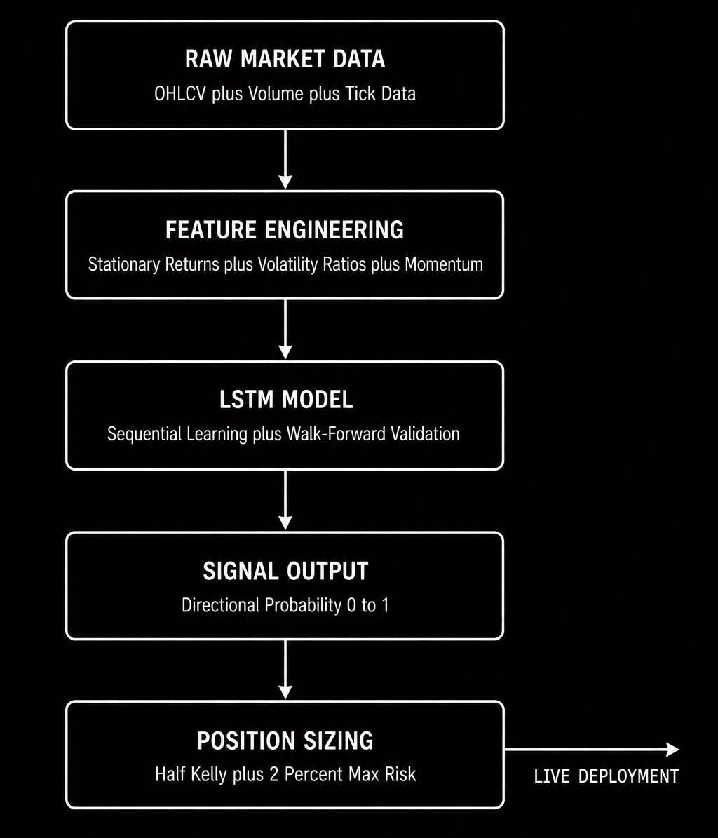
The end-to-end neural network trading signal pipeline from raw data to live position sizing.
This section takes everything from the previous four parts and assembles it into a production-ready signal pipeline. This is the complete end-to-end implementation.
Step 1: Data acquisition and cleaning
Use Polygondotio for institutional-grade tick and OHLCV data. For learning, yfinance is sufficient. Handle missing data, corporate actions, and splits before any feature engineering.
import yfinance as yf
import pandas as pd

ticker = yf.Ticker("SPY")
df = ticker.history(period="5y", interval="1d")
df = df[['Open', 'High', 'Low', 'Close', 'Volume']].copy()
df.dropna(inplace=True)
Step 2: Feature engineering
Build your complete stationary feature set. Every feature must pass the Augmented Dickey-Fuller test.
def build_features(df):
    features = pd.DataFrame(index=df.index)

    close = df['Close']
    volume = df['Volume']
    returns = close.pct_change()

    features['return_1d'] = returns
    features['return_5d'] = close.pct_change(5)
    features['return_20d'] = close.pct_change(20)

    vol_5 = returns.rolling(5).std()
    vol_20 = returns.rolling(20).std()
    features['vol_ratio'] = vol_5 / vol_20
    features['momentum_norm'] = returns / vol_20

    features['volume_zscore'] = (
        (volume - volume.rolling(20).mean()) / volume.rolling(20).std()
    )

    high_low_range = (df['High'] - df['Low']) / close
    features['range_norm'] = high_low_range / high_low_range.rolling(20).mean()

    sma_5 = close.rolling(5).mean()
    sma_20 = close.rolling(20).mean()
    features['sma_ratio'] = sma_5 / sma_20 - 1

    target = (returns.shift(-1) > 0).astype(int)

    features = features.dropna()
    target = target.loc[features.index]

    return features, target
Step 3: Sequential split and scaling
def prepare_data(features, target, lookback=10, train_ratio=0.6, val_ratio=0.2):
    n = len(features)
    train_end = int(n * train_ratio)
    val_end = int(n * (train_ratio + val_ratio))

    scaler = StandardScaler()
    features_scaled = scaler.fit_transform(features[:train_end])

    features_array = np.vstack([
        features_scaled,
        scaler.transform(features[train_end:val_end]),
        scaler.transform(features[val_end:])
    ])

    X, y = prepare_sequences(features_array, target.values, lookback)

    X_train = torch.FloatTensor(X[:train_end - lookback])
    y_train = torch.FloatTensor(y[:train_end - lookback])
    X_val = torch.FloatTensor(X[train_end - lookback:val_end - lookback])
    y_val = torch.FloatTensor(y[train_end - lookback:val_end - lookback])
    X_test = torch.FloatTensor(X[val_end - lookback:])
    y_test = torch.FloatTensor(y[val_end - lookback:])

    return X_train, y_train, X_val, y_val, X_test, y_test, scaler
Step 4: Model evaluation
Beyond directional accuracy, evaluate your model using metrics that matter for trading.
from sklearn.metrics import accuracy_score, roc_auc_score
import pandas as pd

def evaluate_trading_signal(predictions, actuals, returns):
    pred_direction = (predictions > 0.5).astype(int)

    accuracy = accuracy_score(actuals, pred_direction)
    auc = roc_auc_score(actuals, predictions)

    signal = np.where(pred_direction == 1, 1, -1)
    strategy_returns = signal * returns

    sharpe = strategy_returns.mean() / strategy_returns.std() * np.sqrt(252)

    cumulative = (1 + strategy_returns).cumprod()
    rolling_max = cumulative.cummax()
    drawdown = (cumulative - rolling_max) / rolling_max
    max_drawdown = drawdown.min()

    print(f"Directional Accuracy: {accuracy:.4f}")
    print(f"AUC-ROC: {auc:.4f}")
    print(f"Annualized Sharpe: {sharpe:.4f}")
    print(f"Maximum Drawdown: {max_drawdown:.4f}")

    return accuracy, sharpe, max_drawdown
Step 5: Signal to position sizing
A neural network signal alone is not a trading strategy. You need position sizing. The Kelly fraction translates your model’s edge into an optimal bet size:
f* = (p × b - q) / b
Where p is your directional accuracy, q = 1 - p, and b is the average win-to-loss ratio. In practice, use half Kelly to account for parameter estimation error. Never risk more than 2 percent of capital on a single signal regardless of what Kelly recommends.
Step 6: Continuous monitoring and retraining
A model trained on historical data begins degrading the moment it is deployed. Market regimes shift. The conditional expectation the model learned becomes a progressively worse approximation of the current expectation. You must implement a monitoring system that tracks live performance against your validation baseline and triggers retraining when the distribution has shifted beyond an acceptable threshold.
The standard metric is the Kolmogorov-Smirnov statistic comparing your recent live prediction distribution to the historical validation distribution. When the KS statistic exceeds 0.1, retrain on the most recent data and re-evaluate before continuing to deploy.
For prediction markets and crypto specifically, regime shifts are more frequent and more violent than in equity markets. Retraining on a rolling 90-day window with walk-forward re-evaluation every 30 days is a reasonable baseline.
The Summary
Neural networks do not give you a crystal ball. What they give you is a systematic, mathematically rigorous framework for extracting the conditional expectation of market behavior from historical data. When the features are stationary, the architecture is appropriate for sequential data, the training is disciplined and validated correctly, and the signal is sized with proper position management, the result is an edge that is consistent, scalable, and reproducible.
Two Sigma runs 10,000 signals simultaneously through this framework. Renaissance built the highest returning fund in financial history on it. The entry level researcher implementing it earns $650,000 per year.
The complete implementation is in this article. The mathematics is learnable. The code is buildable in a weekend. The only thing that separates the systematic funds from everyone else is knowing the correct framework and the discipline to follow it without cutting corners.
Now you know the framework.
Here is the question I want you to sit with.
A neural network trained on your current indicator set will learn the conditional expectation of market returns given those indicators. But the conditional expectation is only as good as the features you condition on. If you had to add exactly one new feature to your model that you believe no other systematic trader is using, what would it be and why?
Drop your answer in the comments.
There is no wrong answer but there are very revealing ones.
Source
Written by @RohOnChain · View original post